Chapter 1: Land Cover Impacts on Storm Water Runoff and Water Quality
Data and Model Calibration
The hourly weather data were derived from a local weather station at Buffalo Niagara International Airport (USAF-WBAN 725280-14733). Tree and impervious cover parameters (Table 1.1) were derived for the watershed from i-Tree Canopy (i-Tree, 2011), which has users photo-interpret Google Earth imagery (image date circa 2019) to classify points within an area of interest. The tool generated 300 points randomly located within the watershed to bring standard error below 3%. Tree canopy leaf area index (LAI) was estimated at 4.7 based on various field studies.
| Impervious | Tree/Shrub Over Pervious | Tree/Shrub Over Impervious | Grass/Herbaceous | Bare Soil | Surface Water |
|---|---|---|---|---|---|
| 11 | 49.3 | 0.7 | 36.7 | 1.7 | 0.7 |
The model was calibrated using hourly stream flow data collected at the Ellicott Creek gauging station (USGS 04218518) from 10/1/2012-9/30/2013. Model results were calibrated against measured stream flow to yield the best fit between model and measured stream flow results. Calibration coefficients (ranging from -infinity to +1) were calculated for peak flow, baseflow, and balanced flow (peak and base) (Table 1.2). A calibration coefficient of +1 indicates the model predicts a perfect fit with observed data, 0 indicates the model predicts the same as using the mean of observed data, and negative values indicate using the mean of observed data is a better predictor than the model (Moriasi et al., 2007).
| Peak Flow | Base Flow | Balanced Flow |
|---|---|---|
| 0.56 | 0.62 | 0.42 |
Model calibration procedures adjust several model parameters (mostly related to soils) to find the best fit between observed and modeled stream flow on an hourly basis (Figure 1.1). However, there are often mismatches between the precipitation data, which are often collected outside of the watershed, and the actual precipitation that occurs within the watershed. Even if the precipitation measurements are within the watershed, local variations in precipitation intensity can lead to differing amounts of precipitation than observed at the measurement station. These differences in precipitation can lead to poorer fits between the observed and predicted estimates of flow, particularly for peak flow, as the precipitation is a main driver of the stream flow. The divergence of observed and simulated stream flow results (Figure 1.2) is often an artifact of the precipitation data. For example, observed flow will rise sharply, but predicted flow does not, which is an indication of rain in the watershed, but not at the precipitation measurement station. Conversely, the simulated flow may rise but the observed flow does not, which is an indication of rain at the precipitation station, but not in the watershed.
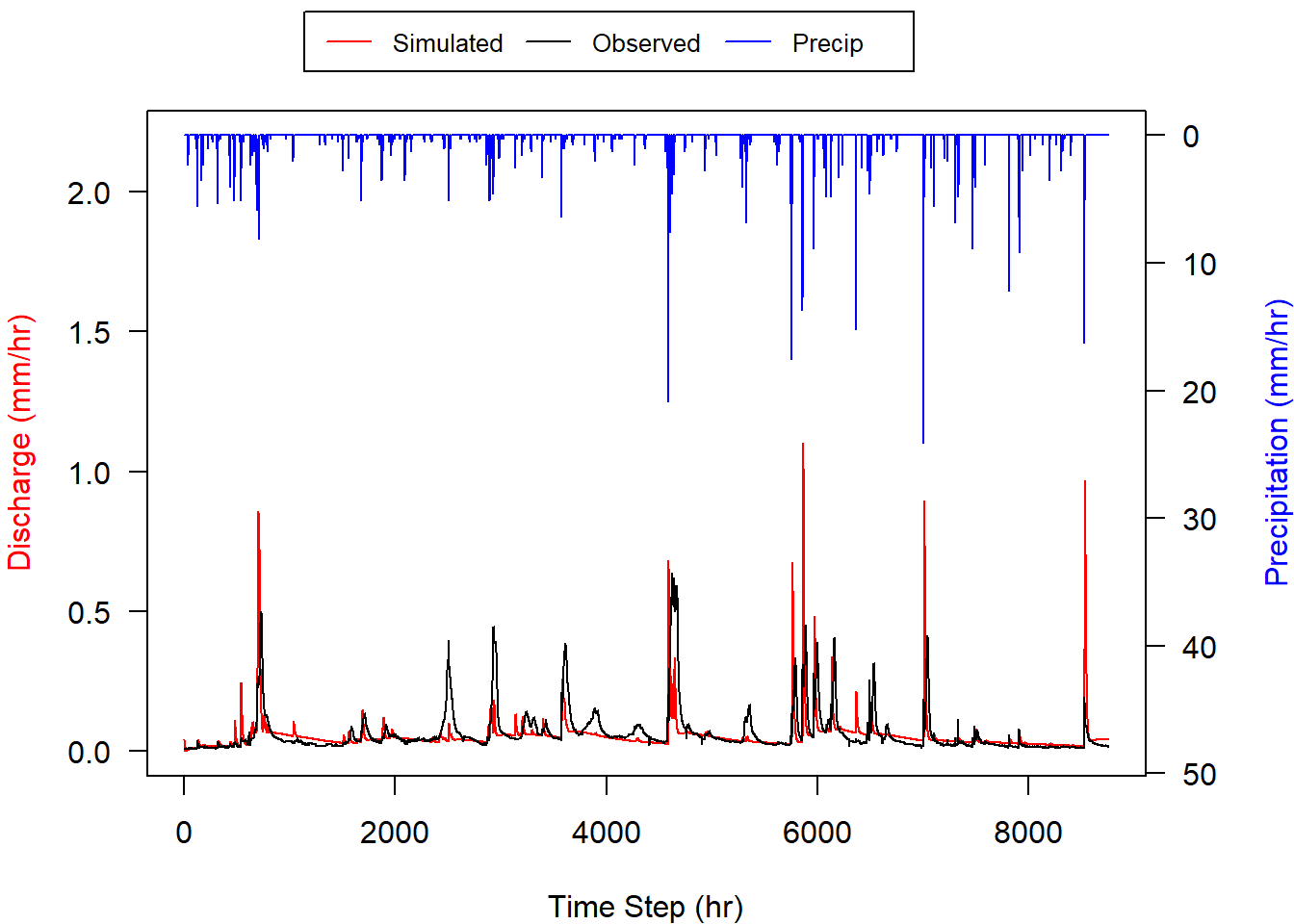

Figure 1.2. Comparison of observed vs. simulated flow.
In watersheds experiencing snowfall, the model processes of snow accumulation, melting, and contribution to surface runoff can also cause divergence between observed and simulated stream flow. During spring thawing, snowmelt runoff is a substantial component of the hydrologic cycle in the cold and snowy climates of the Great Lakes basin. In these months small rain events can generate large responses in stream flow because of the accelerated snowmelt caused by rain falling directly on snow (USDA National Engineering Handbook, 2004). During warmer months, larger rain events will generate relatively smaller responses in stream flow because runoff is no longer supplemented by snowmelt. The Hydro model has computational routines that account for snow accumulation and melting, but traditionally these natural processes are difficult to model and predict because of the complex and variable energy sources (temperature, wind, solar radiation, etc.) contributing to snowmelt (USDA National Engineering Handbook). In these cases model calibration can struggle to fit one set of parameters to two different rainfall-to-runoff relationships: one relationship for months with snowmelt, and one for months without.
Since the model simulations are comparisons between the base simulation stream flows and another simulated flow where surface cover is changed (e.g., increase or decrease in tree cover), both model runs are using the same simulation parameters. This means that the effects of changes in cover types are comparable but may not exactly match the flow of the stream. Stated in another way, the estimates of the changes in surface runoff and stream flow are reasonable (e.g., the relative amount of increase or decrease in runoff are sound as both are using the same model parameters and precipitation data), but the absolute estimate of runoff may be incorrect. The model can be used to compare the relative changes in runoff (e.g., increased tree cover leads to an X% change in runoff) but simulated stream flow will likely not exactly match observed stream flow. The model is more diagnostic of cover change effects than predictive of absolute volumes due to imperfections of models and data used in the model.
Model Scenarios
After calibration, the model was run under various conditions to determine surface runoff response given varying tree and impervious cover values for the watershed area. For tree cover scenarios, impervious cover was held constant at the original value with tree cover varying between 0 and 100 percent. Increasing tree cover was assumed to fill grass and herbaceous covered areas first, followed by bare soil spaces next, and then finally impervious land cover. At 100 percent tree cover, all impervious land is covered by trees. This assumption is unreasonable as all buildings, roads, and parking lots would be covered by trees, but the results illustrate the potential impact. Tree cover reductions assumed that trees were replaced with grass and herbaceous cover.
For impervious cover scenarios, tree cover was held constant with impervious cover varying between 0 and 100 percent. Increasing impervious cover was assumed to fill grass and herbaceous covered areas first, followed by bare soil spaces next and then under tree canopies. The assumption of 100 percent impervious cover is unreasonable, but the results illustrate the potential impact. In addition, as impervious increased from the current conditions, so did the percent of the impervious cover directly connected to the stream, following equations by Sutherland (2000), such that at 100% impervious cover, all impervious cover (100%) is connected to the stream. The percentage of directly connected impervious cover represents the portion of impervious cover that drains directly via overland or through a storm sewer network to the modeled stream or any of its tributaries. Reductions in impervious cover were assumed to be filled with grass and herbaceous cover.
In addition, the model was run while varying both tree and impervious cover from 0 to 100 percent within 10 percent increments to illustrate how varying the amounts of tree and impervious cover affect surface runoff. That is, the model was run at 0 percent tree and 0 percent impervious cover, then 0 percent tree and 10 percent impervious cover, 0 percent tree and 20 percent impervious cover, etc., until all possible combinations were run up to 100 percent tree and 100 percent impervious cover. This results in 11 sets of 11 runs, yielding a total of 121 additional model scenarios. The scenarios described in this section are depicted visually in Figure 1.3.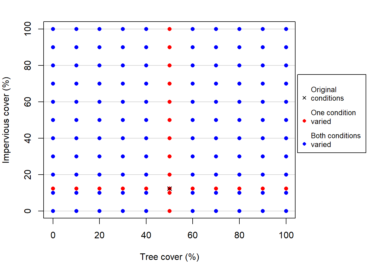
Figure 1.3. Hydro simulations in this study plotted as a function of their amounts of tree cover (%) and impervious cover (%). ‘One condition varied’ represents both the tree cover and impervious cover scenarios described above, and ‘Both conditions varied’ represents the range of 121 scenarios described above.
Water Quality Effects
Event mean concentration (EMC) data are used for estimating pollutant loading into watersheds. EMC is a statistical parameter representing the flow-proportional average concentration of a given parameter during a storm event and is defined as the total constituent mass divided by the total runoff volume. EMC estimates are usually obtained from a flow-weighted composite of concentration samples taken during a storm. Mathematically (Sansalone and Buchberger, 1997; Charbeneau and Barretti, 1998):
(Eq. 1)
where C and Q are the time (t)-variable concentration and flow measured during the runoff event, and M and V are pollutant mass and runoff volume as defined in Equation 1. The EMC values result from a flow-weighted average, not simply a time average of the concentration. EMC data are used for estimating pollutant loading into watersheds. EMCs are reported as a mass of pollutant per unit volume of water (usually mg/L). The pollution Load (L, mass/time) calculation from the EMC method is
(Eq. 2)
where EMC is event mean concentration (mass/volume), Q is runoff of a time period associated with EMC (volume/time), dy is runoff depth of unit area (length/time), and A is the land area (length2) which is the catchment area in i-Tree Hydro. Thus, when the EMC is multiplied by the runoff volume, an estimate of the pollution loading to the receiving water is provided. The instantaneous concentration during a storm can be higher or lower than the EMC, but the use of the EMC as an event characterization replaces the actual time variations of concentration in a storm with a constant concentration having equal mass during the event. This process ensures that mass loadings from storms will be correctly represented. EMCs represent the concentration of a specific pollutant contained in storm water runoff coming from a particular land use type or from the whole watershed. Under most circumstances, the EMC provides the most useful means for quantifying the level of pollution resulting from a runoff event (USEPA, 2002). Figure 1.4 illustrates the inter-storm variation of pollutographs and EMC.
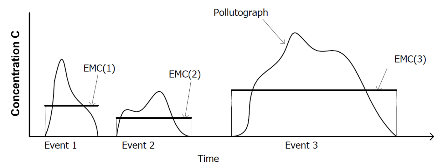
Figure 1.4. Interstorm variation of pollutographs and EMCs.
Since collecting the data necessary for calculating site-specific EMCs can be cost-prohibitive, researchers or regulators will often use values that are already available in the literature. If site-specific numbers are not available, regional or national averages can be used, although the accuracy of using these numbers is questionable. Due to the specific climatological and physiographic characteristics of individual watersheds, agricultural and urban land uses can exhibit a wide range of variability in nutrient export (Beaulac and Reckhow, 1982).
To understand and control urban runoff pollution, the U.S. Congress included the establishment of the Nationwide Urban Runoff Program (NURP) in the 1977 Amendments of the Clean Water Act (PL 95-217). The U.S. Environmental Protection Agency developed the NURP to expand the state knowledge of urban runoff pollution by applying research projects and instituting data collection in selected urban areas throughout the country.
In 1983, the U.S. Environmental Protection Agency (USEPA, 1983) published the results of the NURP, which nationally characterizes urban runoff for 10 standard water quality pollutants, based on data from 2,300 station-storms at 81 urban sites in 28 metropolitan areas.
Subsequently, the USGS created another urban storm water runoff database (Driver et al., 1985), based on data measured through the mid-1980s for over 1,100 stations at 99 urban sites located in 22 metropolitan areas. Additionally, many major cities in the United States collected urban runoff quality data as part of the application requirements for storm water discharge permits under the National Pollutant Discharge Elimination System (NPDES). The NPDES data are from over 30 cities and more than 800 station-storms for over 150 parameters (Smullen et al., 1999).
The data from the three sources (NURP, USGS and NPDES) were used to compute new estimates of EMC population means and medians for the 10 pollutants with many more degrees of freedom than were available to the NURP investigators (Smullen et al., 1999). A “pooled” mean was calculated representing the mean of the total population of sample data. The NURP and pooled mean EMCs for the 10 constitutes are listed in Table 1.3 (Smullen et al., 1999). NURP or pooled mean EMCs were selected because they are based on field data collected from thousands of storm events. These estimates are based on nationwide data, however, so they do not account for regional variation in soil types, climate, and other factors.
| Constituent | Data Source | Mean | Median | Number of Events |
|---|---|---|---|---|
| Total Suspended Solids (TSS) | Pooled | 78.4 | 54.5 | 3047 |
| NURP | 17.4 | 113 | 2000 | |
| Biochemical Oxygen Demand (BOD5) | Pooled | 14.1 | 11.5 | 1035 |
| NURP | 10.4 | 8.39 | 474 | |
| Chemical Oxygen Demand (COD) | Pooled | 52.8 | 44.7 | 2639 |
| NURP | 66.1 | 55 | 1538 | |
| Total Phosphorus (TP) | Pooled | 0.315 | 0.259 | 3094 |
| NURP | 0.337 | 0.266 | 1902 | |
| Soluble Phosphorus (Sol P) | Pooled | 0.129 | 0.103 | 1091 |
| NURP | 0.1 | 0.078 | 767 | |
| Total Kjeldahl Nitrogen (TKN) | Pooled | 1.73 | 1.47 | 2693 |
| NURP | 1.67 | 1.41 | 1601 | |
| Nitrite and Nitrate (NO2 and NO3) | Pooled | 0.658 | 0.533 | 2016 |
| NURP | 0.837 | 0.666 | 1234 | |
| Copper (Cu) | Pooled | 0.0135 | 0.0111 | 1657 |
| NURP | 0.0666 | 0.0548 | 849 | |
| Lead (Pb) | Pooled | 0.0675 | 0.0507 | 2713 |
| NURP | 0.175 | 0.131 | 1579 | |
| Zinc (Zn) | Pooled | 0.162 | 0.129 | 2234 |
| NURP | 0.176 | 0.14 | 1281 |
Note:
1. Pooled data sources include: NURP, USGS, NPDES
2. No BOD5 data available in the USGS dataset - pooled includes NURP+NPDES
3. No TSP data available in NPDES dataset - pooled includes NURP+USGS
A novel approach used in this study is the localization of pollutant coefficient data for three pollutants that were otherwise covered in Table 1.3. National Land Cover Database (NLCD) and HUC-8 basin specific data from White et al. (2015) were used to compute more localized estimates of pollutant coefficient means and medians for 3 pollutants within forest, agriculture and developed NLCD classes (Stephan et al. 2017). These local coefficients were developed for: sediments (equivalent to and replacing TSS from Table 1.3); nitrogen (equivalent to TKN and replacing TKN, NO2 and NO3 from Table 1.3); and phosphorus (equivalent to TP and replacing TP and Soluble P from Table 1.3). White et al. (2015) used sophisticated modeling techniques to estimate water quality data at all HUC-8 watersheds in the contiguous US (about 2,200 total) based on 45 million stochastic Soil and Water Assessment Tool (SWAT) simulations. Those simulations varied climate, topography, soils, weather, land use, management, and conservation implementation conditions to estimate export coefficient values, and the simulations were successfully validated with edge-of-field monitoring data collected at 60 sites from the MANAGE database (Harmel et al., 2006, 2008). Stephan et al. (2017) derived mean and median pollutant coefficients for each HUC-8 based on NLCD data and the runoff water quality data from the White et al. (2015) simulations. Table 1.4 contains the localized pollutant coefficients for the watershed in this report.
Table 1.4. Localized pollutant coefficients (mg/L) based on White et al. (2015) and Stephan et al. (2017). Estimates of absolute reduction in pollutant loads, based on the median values shown here, are included in Table 1.5.
| Minimum | Low | Median | High | Maximum | |
|---|---|---|---|---|---|
| TSS | 19.14 | 40.21 | 147.72 | 494.77 | 778.58 |
| TP | 0.05 | 0.09 | 0.27 | 0.63 | 0.92 |
| TN | 1.18 | 2.20 | 4.25 | 7.49 | 10.18 |
Due to the nature of the White et al. (2015) study, these pollutant coefficients would be considered maximum amounts potentially passing through a watershed stream gauge. For example, with sediment, once sediment is moved by runoff toward the area’s outlet, processes occur (e.g., gravitational settling) that may reduce the amount of suspended sediment that ultimately reaches the area’s outlet. The actual versus potential amount of sediment delivery is referred to as the Sediment Delivery Ratio (SDR). Our modeling approach is designed for comparative analyses that examine how land cover affects sediment load, and to simplify the approach we do not account for SDR within the stream and thus present results as maximum potential values for each statistic.
The national pooled median and mean EMC values for biological and chemical oxygen demand, and copper (Table 1.3), and local land-cover based EMC values for sediment, nitrogen, and phosphorus (Table 1.4), were applied to the change in runoff (pervious and impervious surface flow) due to existing tree cover as compared to a scenario with no tree cover. This process estimates the reduction in pollutant load across the entire modeling time frame. Local management actions (e.g., street sweeping) can affect these values by altering the pollutant loads. However, across the entire season, if the pollutant coefficient value is representative of the watershed, the estimate of cumulative effects on water quality should be relatively accurate. Accuracy of pollution estimates is generally increased by using locally derived coefficients. It is not known how well the national or localized pollutant coefficient values used in this study represent local conditions. The predicted pollutant loading will likely not exactly match absolute amounts of loading measured in the stream.
Results
Tree Cover Effects
Removal of all current tree cover in the Ellicott Creek watershed would increase runoff during the simulation period by an average of 2.5% or 82 million m3. Increasing canopy cover from 50% to 50.0% would reduce runoff by 0% (0.054 million m3) during this 12-month period (Figure 1.5). Increasing tree cover reduces runoff generated from impervious areas and pervious land (Figure 1.6). There is increased reduction in runoff when tree cover increases above 90% because the additional tree cover is added over impervious areas rather than pervious areas.
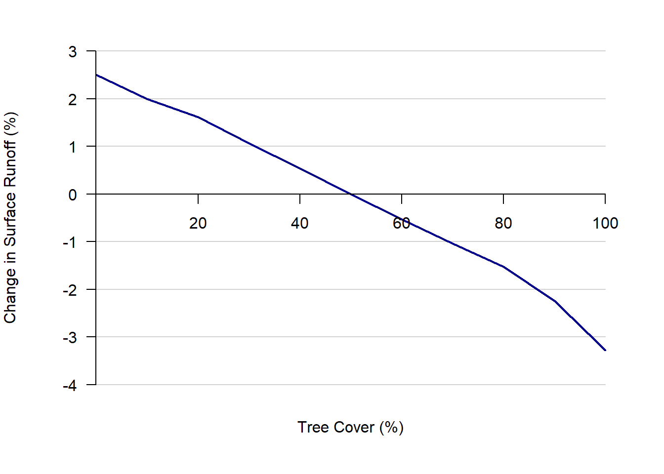
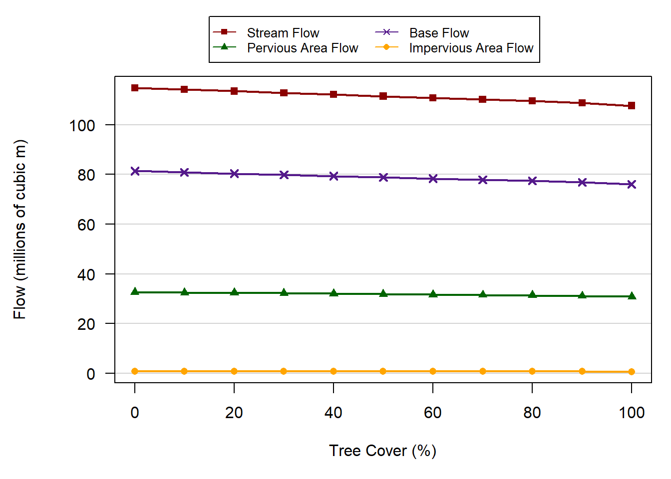
Figure 1.6. Changes in stream flow and components of runoff contributing to stream flow.
Impervious Cover Effects
Removal of all current impervious cover would reduce runoff during the simulation period by an average of 13.6% or 445 million m3. Increasing impervious cover from 12.34% to 60% of the watershed would increase runoff another 170.2% (5.55 billion m3) during this 12-month period (Figure 1.7). Increasing impervious cover reduces baseflow while substantially increasing runoff from impervious surfaces (Figure 1.8).
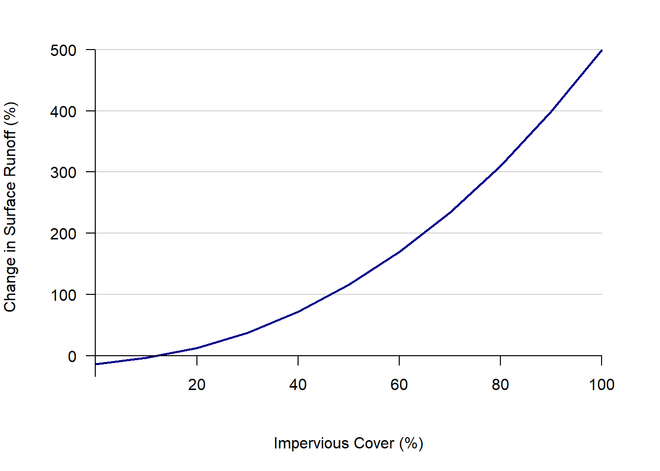
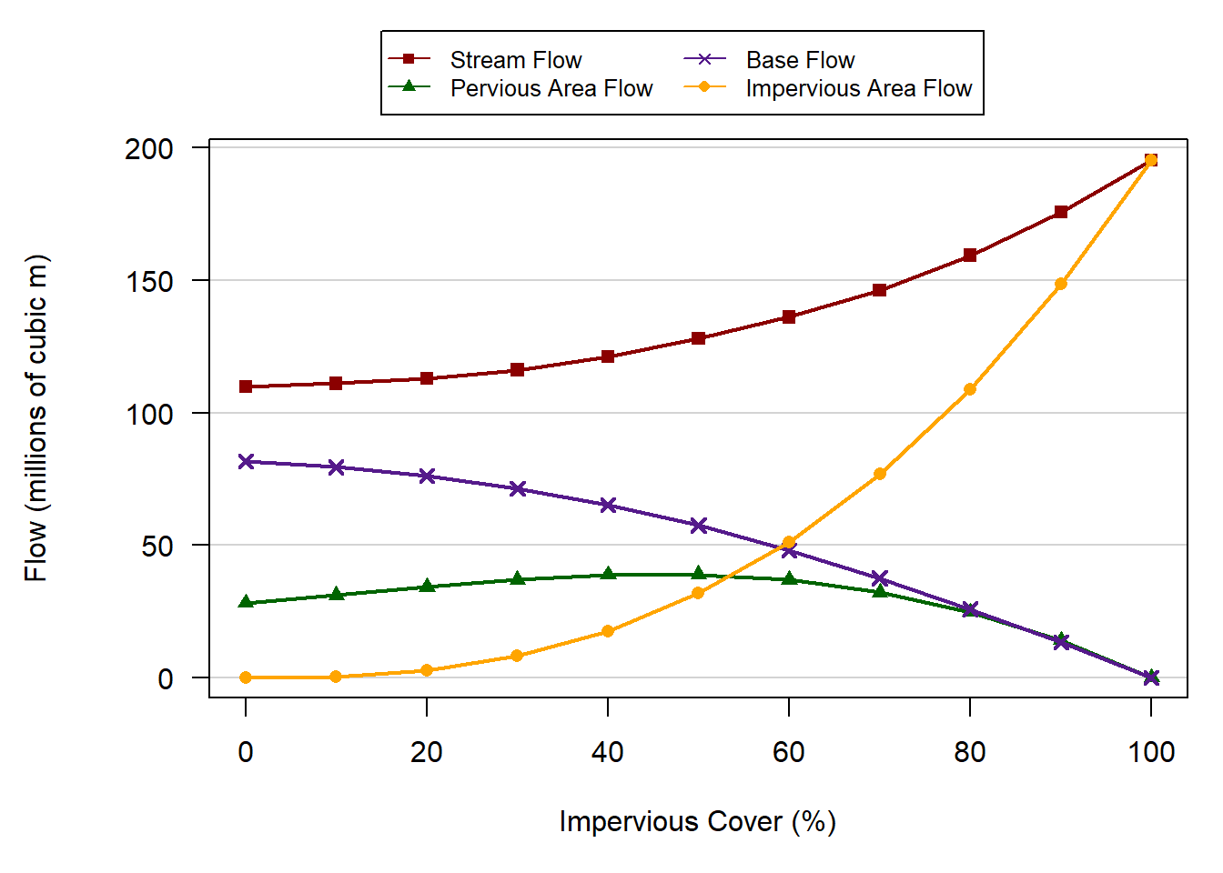
Figure 1.8. Changes in stream flow and components of runoff contributing to stream flow.
Increasing tree cover will reduce runoff, but the dominant cover type influencing runoff is impervious surfaces. Under current cover conditions, increasing impervious cover had a 36.2 times greater impact on runoff relative to tree cover. Increasing impervious cover by 1% averaged a 2.1% increase in runoff, while increasing tree cover by 1% averaged only a 0.058% decrease in runoff. Changes in runoff volume (Figure 1.9) and percent change in runoff (Figure 1.10) vary depending upon the amount of existing tree and impervious cover.

Figure 1.9. Changes in runoff during simulation period based on changes in percent impervious and percent tree cover. White square represents current conditions.
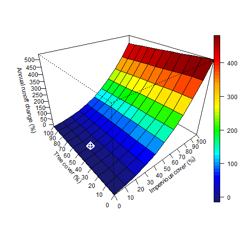
Figure 1.10. Percent change in annual runoff during simulation period based on changes in percent impervious and percent tree cover. White square represents current conditions.
During the simulation period the total rainfall recorded was 111.9 cm. Since that amount is assumed to have fallen over the entire 220.3 km2 watershed, a total of 247 million m3 of rain fell on the watershed during the simulation period. The total stream flow modeled for the simulation period in the base case scenario (no land cover change) was 111 million m3. The stream flow is made up of runoff and baseflow. The greatest contribution to stream flow was baseflow, which was estimated to generate 70.7% of stream flow. Runoff from pervious areas and runoff from impervious areas generated 28.6% and 0.7% of stream flow respectively. Watershed areas with tree canopy intercepted about 9% of the rainfall that fell in those areas; but as only 50% of the watershed is under tree canopy, interception of total precipitation by trees was only 4.5% (11 million m3). Watershed areas with short vegetation cover (grasses and herbaceous vegetation) intercepted about 3.8% of the rainfall that fell in those areas; but as only 36.66% of the watershed has short vegetation cover, interception of total precipitation by short vegetation was only 1.4% (3.5 million m3). About 54.8% of total precipitation is estimated to re-enter the atmosphere through evaporation or evapotranspiration (including evaporation from interception) or go to groundwater recharge.
Effects on Water Quality
Based on the changes in runoff rates and the EMC values used (Tables 1.3 & 1.4), the current tree cover is estimated to reduce total suspended solids during the simulation period by about 121 tonnes. Other pollutants are also reduced (Table 1.5). These are all major pollutants associated with urban runoff and potentially harmful to receiving waters (Horner et al., 1994).
Table 1.5. Estimated reduction in tonnes of water pollutants due to existing tree cover during the simulation period, based on median pooled event mean concentration values.
| Total Suspended Solids | Biochemical Oxygen Demand | Chemical Oxygen Demand | Total Phosphorus | Total Nitrogen | Copper | |
|---|---|---|---|---|---|---|
| Median | 120.693 | 9.396 | 36.522 | 0.219 | 3.477 | 0.009 |
Discussion
Impervious cover is the dominant cover type in affecting runoff in the watershed, with an impact about 36.2 times greater than trees. This value is affected in part by the assumptions for changing tree cover between model scenarios. To isolate the separate effects of both cover types, impervious cover is kept unchanged when tree cover is changed and vice versa. When trees are added to the model they are therefore assumed to cover pervious land first. This produces conservative estimates of the effect of tree cover on runoff and stream flow. This is demonstrated in Figure 1.5: runoff declines more steeply above about 90% tree cover, corresponding to the point where additional trees must begin to be planted over impervious cover. These new trees now intercept precipitation that would otherwise have fallen on the dominant cover type affecting runoff, resulting in a larger response to additional tree cover.
If impervious surfaces cannot be removed from the watershed, adding tree cover to impervious land reduces runoff more effectively than adding tree cover to pervious land (Figure 1.5), so efforts to increase tree cover over impervious lands will maximize tree effects on runoff. If impervious cover can be removed and replaced, replacing with pervious cover in general and pervious with trees in particular would maximize landscape effects on reducing runoff. Tree canopy intercepted 2.4 times more rainfall than short vegetation. Maximizing leaf area with larger trees would maximize the reduction in storm water runoff.
Information from this report can be used to better understand the impacts of tree and impervious cover on runoff, stream flow, and water quality in the Ellicott Creek watershed. Through better landscape designs of both tree and impervious cover, runoff can be reduced and water quality improved in waterways that drain into the Great Lakes.