Land Use Planning Impacts on Near Shore Pollution Loading in the Great Lakes
HUC Report: 04070005
The effects of land cover and urban forests were evaluated in Black as part of the Great Lakes Restoration Initiative (GLRI: https://www.glri.us/) program.This report is intended to provide data and information for local land managers to understand the impact of their current land use on runoff, water quality, and preservation of natural resources. The report is organized as follows:
- Introduction: Area and project metadata
- Buffer: Non-point source pollution mapping and hotspot analysis
- Figures: Collection of all figures used in the report
- Downloads: Access GeoTIFFs of maps
Introduction
|
Subbasin |
|
|
Name: |
Black |
|
HUC8 |
04070005 |
|
Drains to: |
Lake Huron |
|
State(s): |
Michigan |
|
Area: |
1554.01 km2 |
Table 1.1 Subbasin metadata
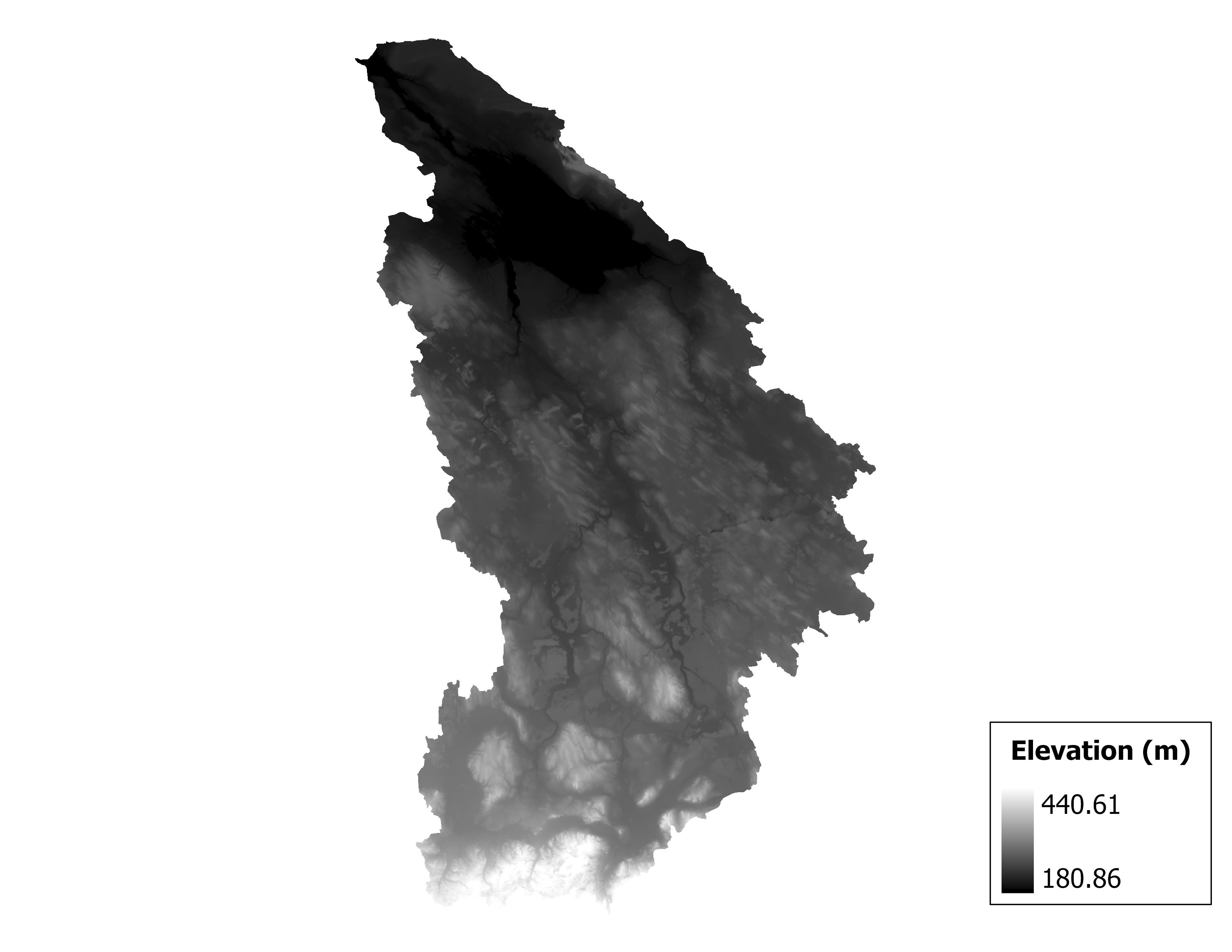
Figure 1.2 Map of elevation in the Black subbasin.
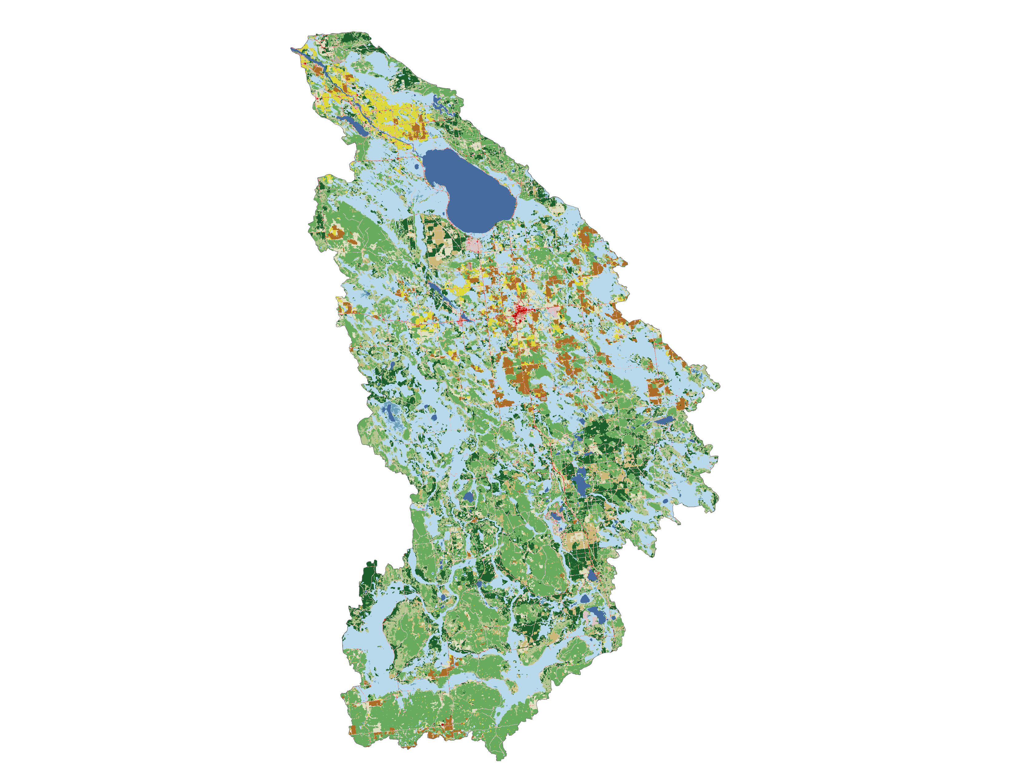

Figure 1.3 Land cover in the Black subbasin.
|
Land Use |
|
|
% Forest |
45.84% |
|
% Agriculture |
5.97% |
|
% Urban |
5.45% |
|
Average % Impervious Cover |
0.8% |
|
Average % Tree Cover |
60.86% |
Table 1.4 Current land use (2019 NLCD)
Nutrient Loading
Data and Methods
The i-Tree Buffer model is built upon the framework of Endreny and Wood (2003) and creates maps of watershed runoff likelihood and buffering likelihood values. This analysis used publicly available GIS inputs, annual rainfall data, and local (White et al., 2015) values for nonpoint source (NPS) loading of nutrients. The GIS inputs include digital elevation model (DEM) data and land use data, retrieved from NHDPlusV2 and National Land Cover Database (NLCD), respectively.
Values for NPS loading were taken from compiled look-up tables of local export coefficient (EC, kg/ha/yr) values (Table 3.1) developed by White et al. (2015), which estimated water quality data at the HUC-8 basin scale nationwide based on 45 million stochastic Soil and Water Assessment Tool (SWAT) simulations. ECs represent the annual loads of a pollutant for a given land cover type, and are empirically derived from observed water quality data from catchments with varying land uses. Land cover types representing permanent water or ice (NLCD classes 11, 12, 90, and 95) were assumed to have ECs of zero.
| Pollutant | NLCDa | 5th percentile | 10th percentile | 25th percentile | 50th percentile | 75th percentile | 90th percentile |
|---|---|---|---|---|---|---|---|
| TP | 21 | 0.378 | 0.416 | 0.492 | 0.621 | 0.796 | 1.47 |
| 22 | 0.378 | 0.416 | 0.492 | 0.621 | 0.796 | 1.47 | |
| 23 | 0.378 | 0.416 | 0.492 | 0.621 | 0.796 | 1.47 | |
| 24 | 0.378 | 0.416 | 0.492 | 0.621 | 0.796 | 1.47 | |
| 41 | 0.0 | 0.0 | 0.0 | 0.0 | 0.019 | 0.032 | |
| 42 | 0.0 | 0.0 | 0.0 | 0.0 | 0.019 | 0.032 | |
| 43 | 0.0 | 0.0 | 0.0 | 0.0 | 0.019 | 0.032 | |
| 71 | 0.0 | 0.015 | 0.033 | 0.062 | 0.097 | 0.153 | |
| 81 | 0.09 | 0.13 | 0.23 | 0.43 | 0.75 | 1.19 | |
| 82 | 0.046 | 0.068 | 0.142 | 0.663 | 1.294 | 2.365 | |
| TN | 21 | 15.023 | 15.837 | 17.144 | 18.964 | 21.581 | 28.224 |
| 22 | 15.023 | 15.837 | 17.144 | 18.964 | 21.581 | 28.224 | |
| 23 | 15.023 | 15.837 | 17.144 | 18.964 | 21.581 | 28.224 | |
| 24 | 15.023 | 15.837 | 17.144 | 18.964 | 21.581 | 28.224 | |
| 41 | 0.601 | 0.671 | 0.803 | 0.958 | 1.14 | 1.497 | |
| 42 | 0.601 | 0.671 | 0.803 | 0.958 | 1.14 | 1.497 | |
| 43 | 0.601 | 0.671 | 0.803 | 0.958 | 1.14 | 1.497 | |
| 71 | 0.453 | 0.563 | 0.886 | 1.44 | 2.199 | 3.19 | |
| 81 | 0.97 | 1.34 | 2.31 | 4.08 | 6.96 | 10.79 | |
| 82 | 1.432 | 1.733 | 2.749 | 9.502 | 18.245 | 25.394 |
Table 3.1 Export coefficients based on percentile and pollutant type (White et al. 2015)
a NLCD land cover classes: 21 - Developed, open space; 22 - Developed, low intensity; 23 - Developed, medium intensity;
24 - Developed, high intensity; 41 - Deciduous forest; 42 - Evergreen forest; 43 - Mixed forest; 71 - Grassland or herbaceous; 81 - Pasture or hay; 82 - Cultivated crops
With these input data, the model calculated:
separate ECs for each pixel;
a separate surface and subsurface runoff index (RI) for each pixel based on the fractions of impervious and pervious area in each upslope contributing area pixel, which is related to an estimate of surface and subsurface wetness; and
a separate surface and subsurface buffer index (BI) for each pixel based on flow resistance and potential energy, which is related to runoff velocity and an estimate of NPS buffering in downslope dispersal area pixels.
The entire set of pixel specific RI and BI values are normalized to the watershed mean RI and BI values (or median values, depending on user preference), and multiplied by the land cover EC to quantify pollutant loading likelihood. In this way i-Tree Buffer treats pollutant loading as spatially variant, depending on both RI from upslope pixels and BI from downslope pixels. As demonstrated in Figure 2.1, changes in RI and BI control pollutant loading through changes in runoff magnitude (i.e., size of arrows under each scenario) and/or pollutant concentration (i.e., the color of arrows under each scenario).

Figure 3.2 Conceptual model of the effects of contributing area RI (a & b) and dispersal area BI (c & d) on NPS loading from a pixel of interest.
Weighted surface and subsurface EC values for each pixel i, or dynamic export coefficients (ECd), are calculated as:
$$EC_{d,surf,i} = EC_{surf,i}*\frac{RI_{surf,i}}{RI_{surf,avg}}*\frac{BI_{surf,avg}}{BI_{surf,i}}$$
(Eq. 1)
$$EC_{d,sub,i} = EC_{sub,i}*\frac{RI_{sub,i}}{RI_{sub,avg}}*\frac{BI_{sub,avg}}{BI_{sub,i}}$$
(Eq. 2)
where ECi represents the unweighted EC (kg/ha/yr) for land cover type i, RIi is the pixel’s surface or subsurface runoff index value, the RIavg is the corresponding average surface or subsurface runoff index in the watershed, the BIi is the pixel’s surface or subsurface buffer index value, and BIavg is the corresponding average surface or subsurface buffer index in the watershed. The NPS pollutant of phosphorus was simulated as total phosphorus entrained in surface runoff processes, denoted as ECsurf,i in Equation 1. The NPS pollutant of nitrogen was simulated as dissolved total nitrogen in subsurface runoff processes, denoted as ECsub,i in Equation 2 (Stephan and Endreny 2016).
Values of ECd for P and N were calculated for the entire watershed and mapped in 30m square pixels. To focus on the most critical watershed areas for possible management and remediation, three hotspots were identified in the watershed for TN, TP, and TSS. Hotspots were calculated by a moving 3x3 window of 30m cells, with a 0.5 km buffer in each direction. In other words, hotspots were gathered by the 3x3 cell average, with no hotspot less than 0.5km away from each other.
Results
Effects of Land Use on Water Quality
Based on the current and potential land use, event mean concentrations (EMCs) were calculated based on White et al. (2015) and plotted into ternary heat maps.
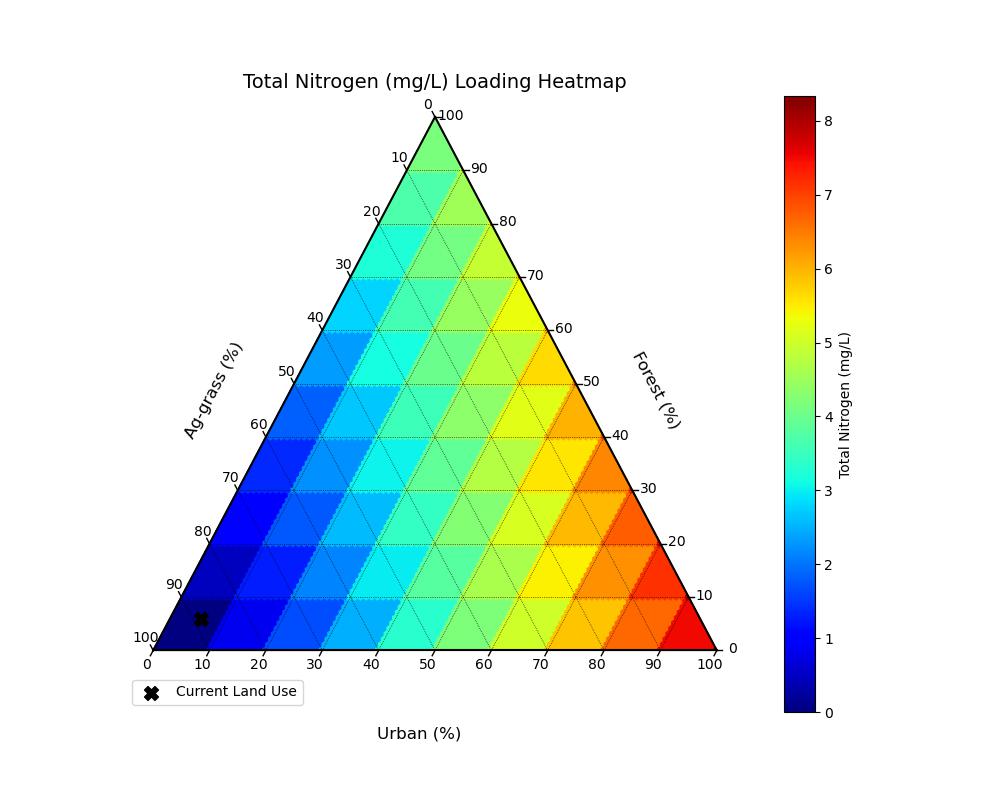
Figure 3.3: Localized pollutant coefficients (mg/L) for Total Nitrogen based on White et al. (2015). Black 'X' represents current conditions.
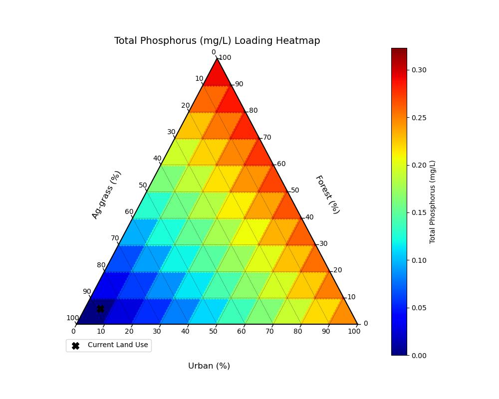
Figure 3.4: Localized pollutant coefficients (mg/L) for Total Phosphorus based on White et al. (2015). Black 'X' represents current conditions.
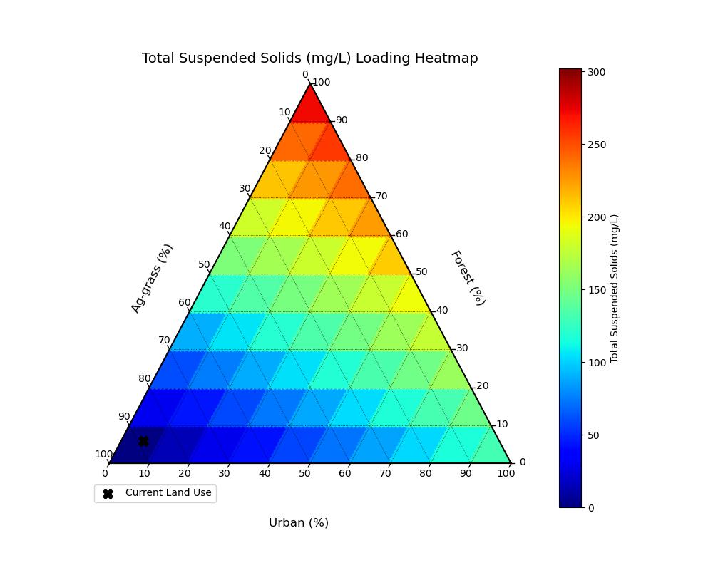
Figure 3.5 Localized pollutant coefficients (mg/L) for Total Suspended Solids based on White et al. (2015). Black 'X' represents current conditions.
Hotspots
The watershed mean loading value was 6.5 kg/ha/yr of total nitrogen (TN) and the standard deviation was 18.82 kg/ha/yr.
Explore the top hotspots for total nitrogen (TN) below:
Or view the images and coordinates for the top 3 hotspots:
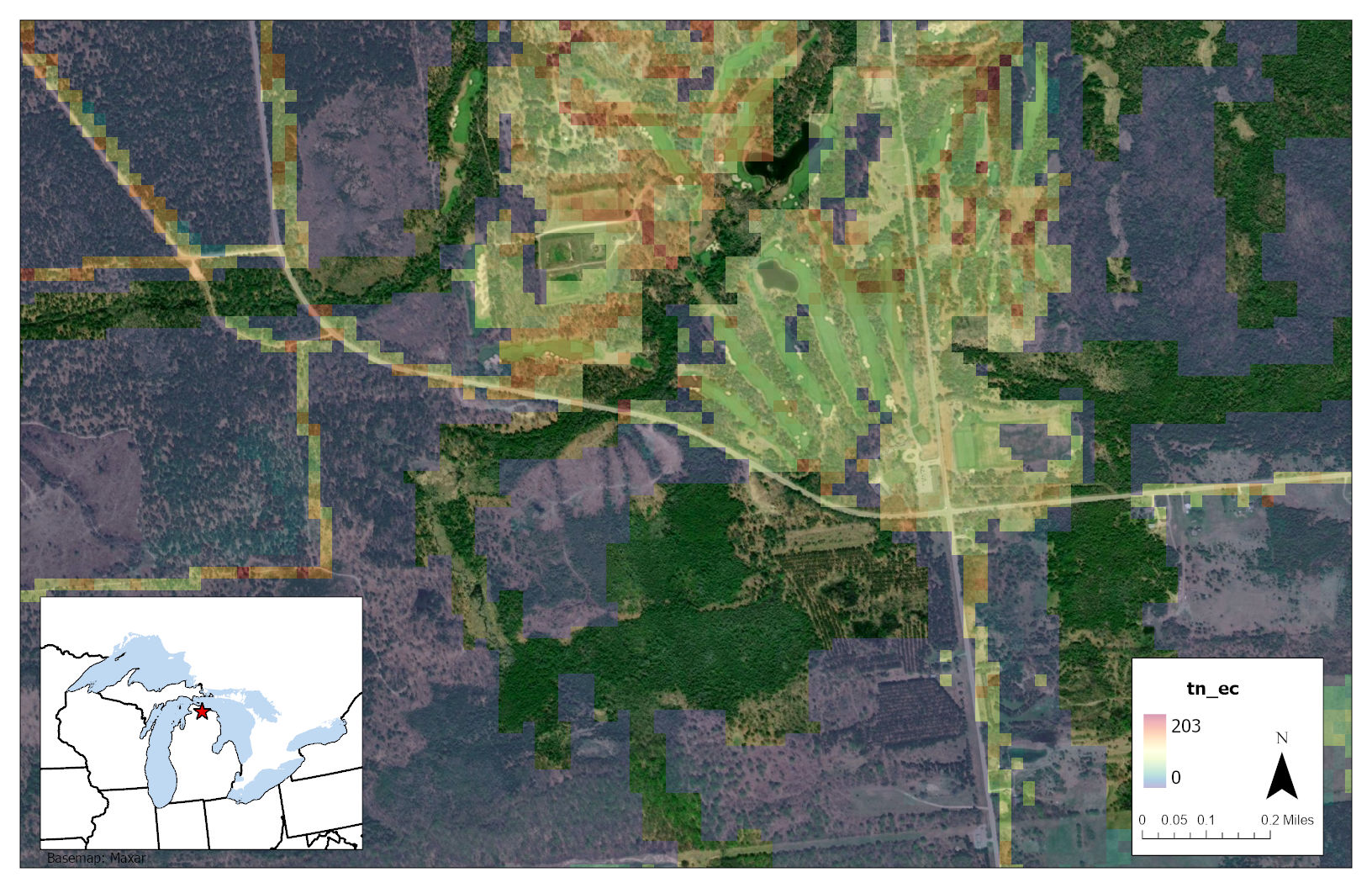
Figure 3.6 Hotspot 1: Latitude:45.41947 Longitude:-84.27484
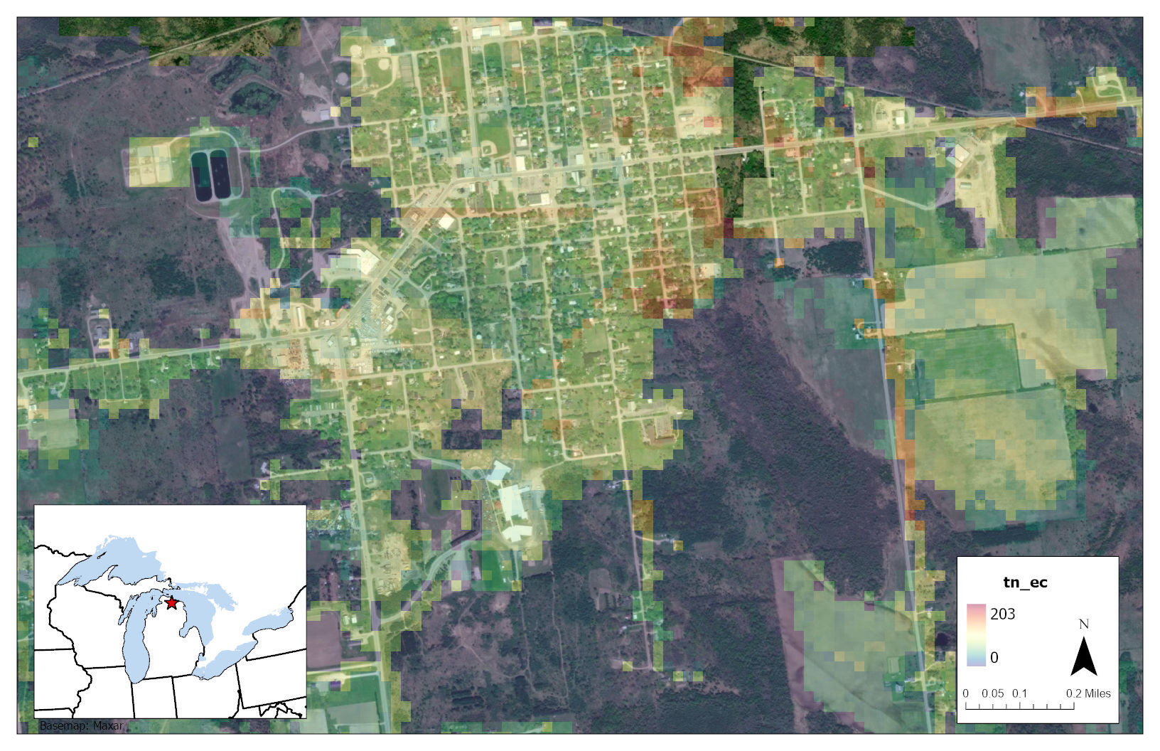
Figure 3.7 Hotspot 2: Latitude:45.35791 Longitude:-84.22392
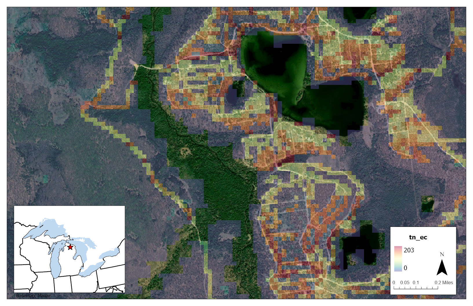
Figure 3.8 Hotspot 3: Latitude:45.1809 Longitude:-84.2205
The watershed mean loading value was 0.2093 kg/ha/yr of total phosphorus (TP) and the standard deviation was 0.61 kg/ha/yr.
Explore the top hotspots for total phosphorus (TP) below:
Or view the images and coordinates for the top 3 hotspots:
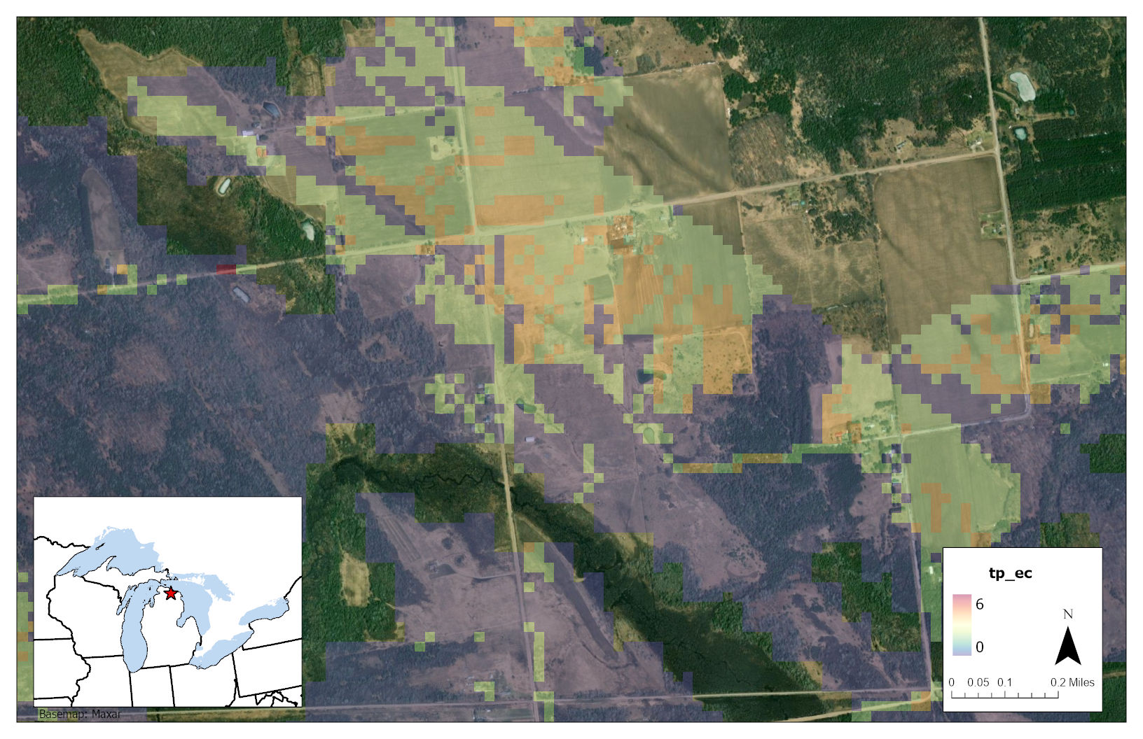
Figure 3.9 Hotspot 1: Latitude:45.34217 Longitude:-84.10707
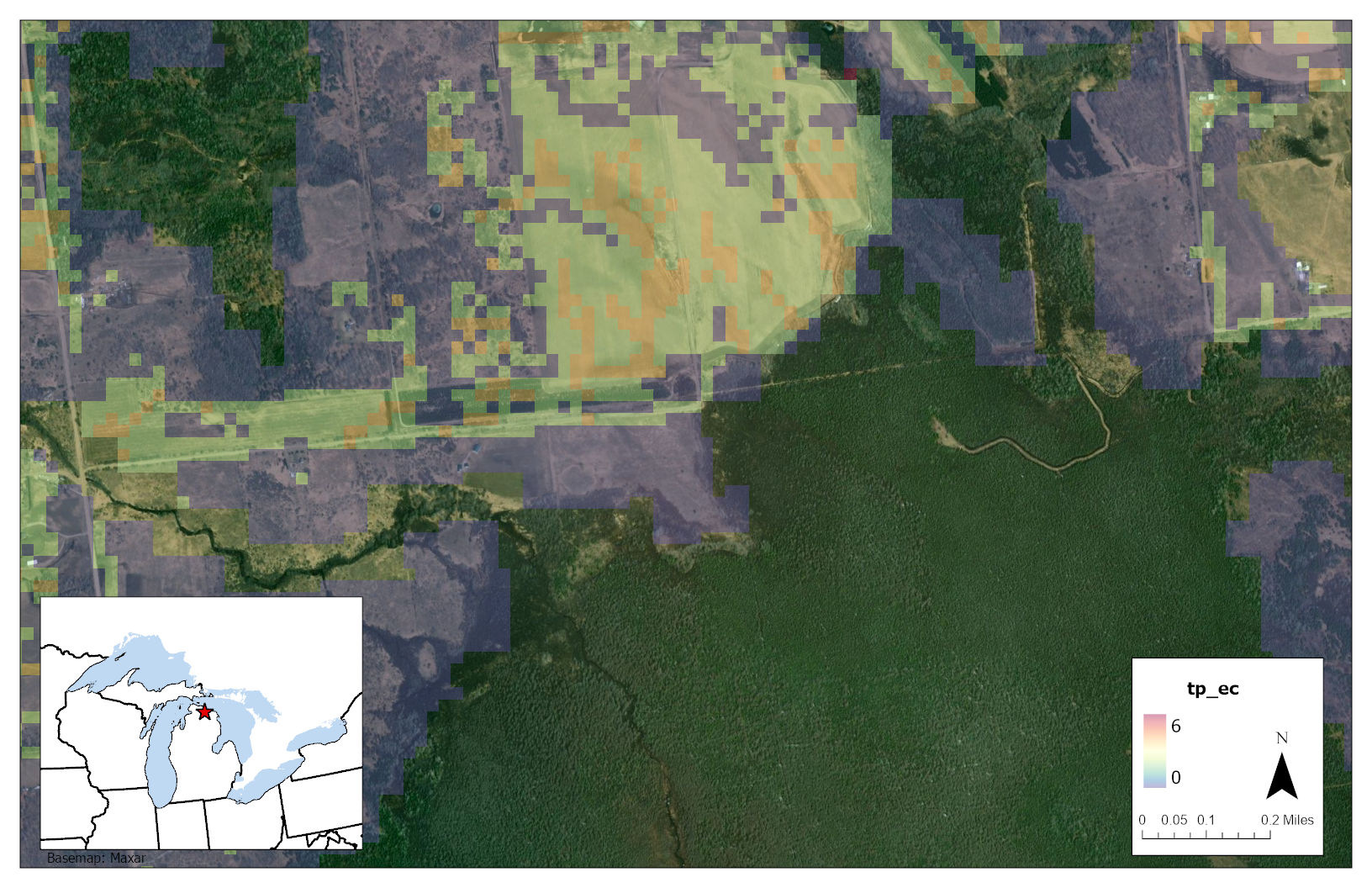
Figure 3.10 Hotspot 2: Latitude:45.38468 Longitude:-84.12651
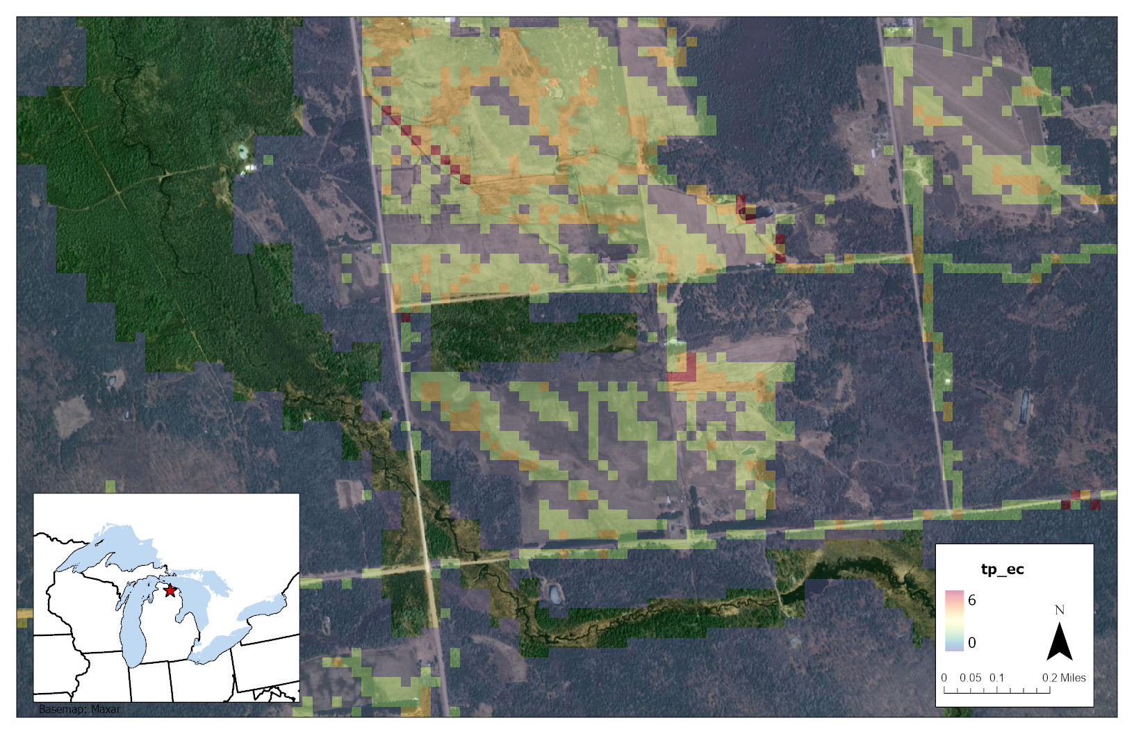
Figure 3.11 Hotspot 3: Latitude:45.27421 Longitude:-84.07678
Discussion
The resolution of the ECd result rasters is constrained by the coarse resolution of the input data, but Buffer can run with 30m pixels and produce maps with useful insight into trends of RI, BI, and ECd. The 30m input data captures flow path tendency toward perennial stream networks while maintaining this study’s first-order modeling approach and providing results closer to the scales at which remediation designs are implemented. For urban basins in particular, the model accuracy can be improved if used with higher resolution elevation and land cover data, since coarser data can miss sub-pixel details of land use and flow paths imposed by features such as road crowns and curbs. However, although Stephan and Endreny (2016) ultimately used <1m input data they saw <1% difference in total nutrient load values between 0.3m and 10m grid sizes.
For each of the critical hotspots, management efforts to reduce NPS nutrient loading could take one of several approaches. General approaches can be divided into three categories:
- Reducing pollutant export at the hotspot. This reduction could involve altering land cover at the hotspot to land cover with a lower NPS loading value or incorporating best management practices into the current land use (e.g., contour farming and covered fertilizer storage in an agricultural hotspot).
- Increasing buffering capacity in the downslope flow path of the hotspot (i.e. raising BI). BI values increase with increasing water travel times in the downslope dispersal area. Travel times could be increased by increasing the percentages of herbaceous and woody vegetation in dispersal area land cover, or by decreasing local terrain slopes.
- Reducing runoff generation upslope of the hotspot (i.e. lowering RI). This reduction could be accomplished by removing impervious cover or decreasing local terrain slopes in the upslope contributing area.
A management plan for a given hotspot could involve any combination of the above approaches. Ultimately, management needs to be tailored to each hotspot’s unique conditions for land cover and land use, topographic index, social conditions, and plantable space. Trees and forests help reduce NPS nutrients through any of the three approaches listed above when planted in the right place for the right reason. These trees would also provide many co-benefits and contribute to sustainable forestry, agroforestry, and ecosystem restoration in these hotspot areas.
All of these management approaches could be further directed by taking plantable space into account. Nutrient hotspot locations can be compared with local plantable space data to strategically target tree plantings that will minimize NPS pollution as well as expand tree canopy in low-canopy areas. Strategic planting of trees has been identified as a crucial component of reducing NPS pollution in both urban and rural watersheds (Sharpley et al., 2006; Hynicka and Caraco, 2017).