Land Use Planning Impacts on Near Shore Pollution Loading in the Great Lakes
HUC Report: 04150101
The effects of land cover and urban forests were evaluated in Black as part of the Great Lakes Restoration Initiative (GLRI: https://www.glri.us/) program.This report is intended to provide data and information for local land managers to understand the impact of their current land use on runoff, water quality, and preservation of natural resources. Current land use is also compared to potential land uses along the shoreline to guide planning and management decisions. The report is organized as follows:
- Introduction: Area and project metadata
- Shoreline: Land cover influences on runoff quantity and quality at shoreline
- Buffer: Non-point source pollution mapping and hotspot analysis
- Figures: Collection of all figures used in the report
- Downloads: Access GeoTIFFs of maps
Introduction
|
Subbasin |
|
|
Name: |
Black |
|
HUC8 |
04150101 |
|
Drains to: |
Lake Ontario |
|
State(s): |
New York |
|
Area: |
4938.97 km2 |
Table 1.1 Subbasin metadata
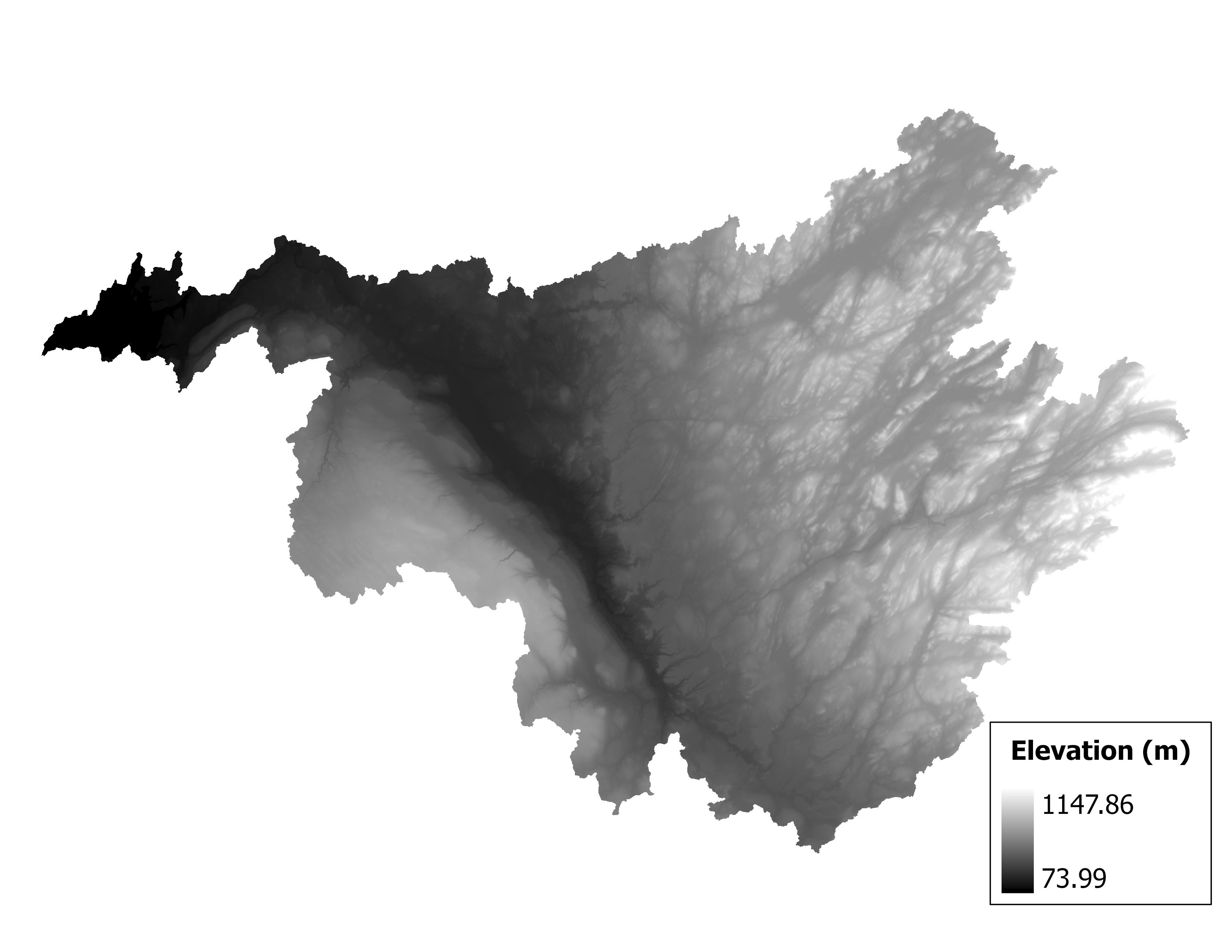
Figure 1.2 Map of elevation in the Black subbasin.
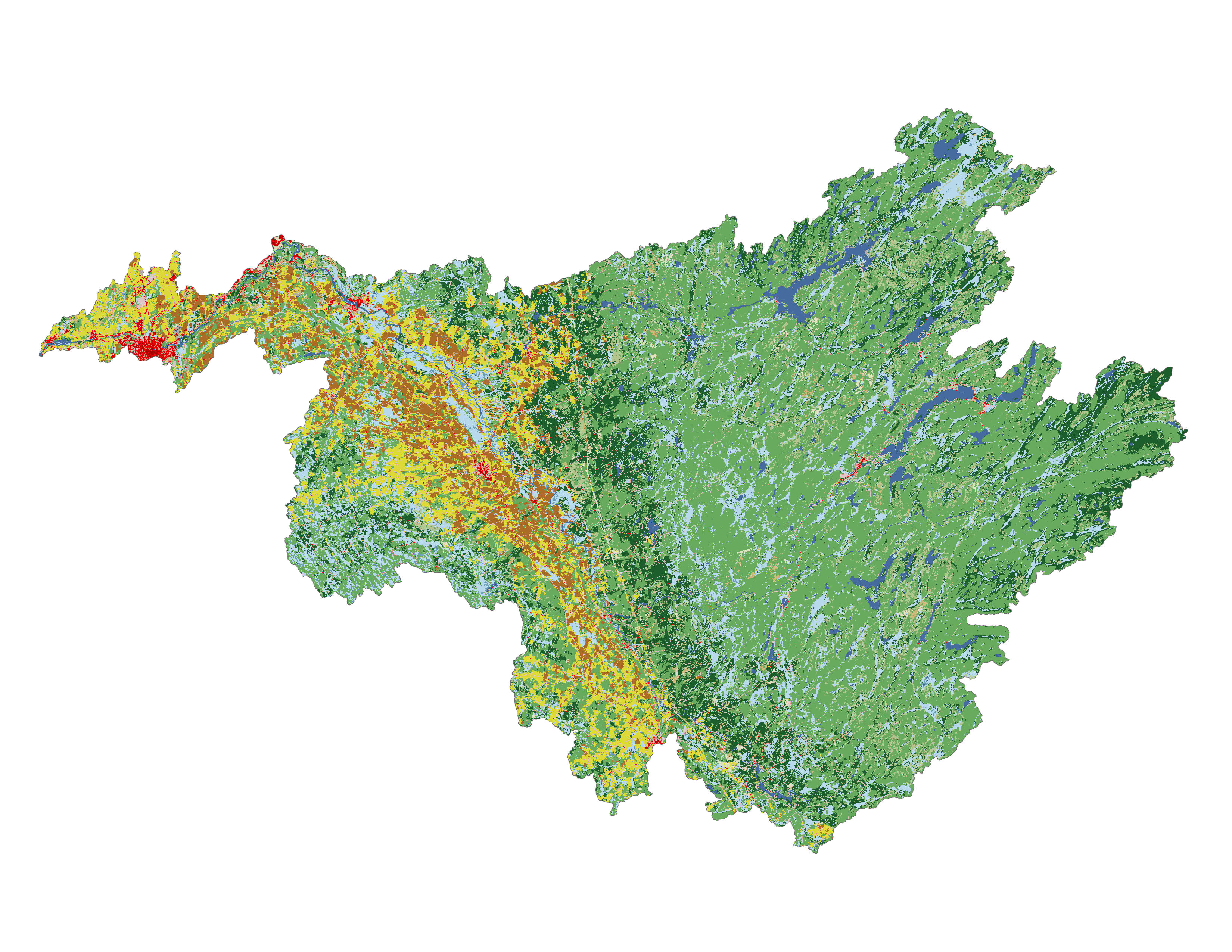

Figure 1.3 Land cover in the Black subbasin.
|
Land Use |
|
|
% Forest |
65.29% |
|
% Agriculture |
12.33% |
|
% Urban |
3.59% |
|
Average % Impervious Cover |
0.82% |
|
Average % Tree Cover |
62.32% |
Table 1.4 Current land use (2019 NLCD)
|
Weather Station |
|
|
Station Name |
GREATER ROCHESTER INTERNATIONAL AP |
|
USAF-WBAN |
725290-14768 |
|
Year Simulated |
2012 |
|
Annual Precipitation |
805.18 mm |
Table 1.5 Weather station metadata
Shoreline
Black subbasin has 1.76 km2 of shoreline area that was analyzed using i-Tree Hydro. Tree and impervious cover parameters (Table 2.1) were derived for the watershed from i-Tree Canopy (i-Tree, 2011), which uses photointerpretation of Google Earth imagery (2021) to classify points within an area of interest. The tool generated 250 points randomly located within the watershed to bring the standard error below 3%.
|
Tree/shrub over pervious
|
Tree/shrub over impervious
|
Impervious
|
Grass/herbaceous
|
Bare soil
|
Surface water
|
|
22.0%
|
13.0%
|
23.0%
|
29.0%
|
13.0%
|
0.0%
|
Table 2.1 i-Tree Canopy Estimates of tree and impervious cover
Previously, model calibration was performed using hourly stream flow data to adjust model parameters for a best fit between observed and modeled stream flow on an hourly basis. However, due to the limits of this calibration and the lack of observed streamflow over a shoreline area, model calibration was done based on the simulation end groundwater at the soil surface. Soil parameters of hydraulic conductivity decay (n), scale parameter of soil transmissivity (m), and initial stream discharge and soil moisture deficit (Q0_mph) were calibrated to reasonable soil saturation at the end of the simulation.
Since the model simulations are comparisons between the base simulation stream flows and another simulated flow where surface cover is changed (e.g., increase or decrease in tree cover), both model runs are using the same simulation parameters. This means the effects of changes in cover types are comparable but may not match the stream's flow.
Stated in another way, the estimates of the changes in surface runoff and stream flow are reasonable (e.g., the relative amount of increase or decrease in runoff are sound as both are using the same model parameters and precipitation data), but the absolute estimate of runoff may be incorrect. The model can be used to compare the relative changes in runoff (e.g., increased tree cover leads to an X% change in runoff) but simulated stream flow will likely not exactly match observed stream flow. The model is more diagnostic of cover change effects than predictive of absolute volumes due to imperfections of models and data used in the model.
Methods
After calibration, the model was run under various conditions to determine surface runoff response given varying tree and impervious cover values for the watershed area. For tree cover scenarios, impervious cover was held constant at the original value with tree cover varying between 0 and 100 percent. Increasing tree cover was assumed to fill grass and herbaceous covered areas first, followed by bare soil spaces next, and then finally impervious land cover. At 100 percent tree cover, all impervious land is covered by trees. This assumption is unreasonable as all buildings, roads, and parking lots would be covered by trees, but the results illustrate the potential impact. Tree cover reductions assumed that trees were replaced with grass and herbaceous cover.
For impervious cover scenarios, tree cover was held constant with impervious cover varying between 0 and 100 percent. Increasing impervious cover was assumed to fill grass and herbaceous covered areas first, followed by bare soil spaces next and then under tree canopies. The assumption of 100 percent impervious cover is unreasonable, but the results illustrate the potential impact. In addition, as impervious increased from the current conditions, so did the percent of the impervious cover directly connected to the stream, following equations by Sutherland (2000), such that at 100% impervious cover, all impervious cover (100%) is connected to the stream. The percentage of directly connected impervious cover (DCIA) represents the portion of impervious cover that drains directly via overland or through a storm sewer network to the modeled stream or any of its tributaries. Reductions in impervious cover were assumed to be filled with grass and herbaceous cover.
In addition, the model was run while varying both tree and impervious cover from 0 to 100 percent within 10 percent increments to illustrate how varying the amounts of tree and impervious cover affect surface runoff. That is, the model was run at 0 percent tree and 0 percent impervious cover, then 0 percent tree and 10 percent impervious cover, 0 percent tree and 20 percent impervious cover, etc., until all possible combinations were run up to 100 percent tree and 100 percent impervious cover. This results in 11 sets of 11 runs, yielding a total of 121 additional model scenarios. The scenarios described in this section are depicted visually in Figure 2.2.

Figure 2.2 Hydro simulations in this study plotted as a function of their amounts of tree cover (%) and impervious cover (%)
National Land Cover Database (NLCD) and HUC-8 basin specific export coefficient data from White et al. (2015) were used to compute more localized estimates of pollutant coefficient means and medians for 3 pollutants within forest, agriculture and developed NLCD classes (Stephan et al. 2017). These local coefficients were developed for: sediments (TSS), nitrogen (TN), and phosphorus (TP). White et al. (2015) used sophisticated modeling techniques to estimate water quality data at all HUC-8 watersheds in the contiguous US (about 2,200 total) based on 45 million stochastic Soil and Water Assessment Tool (SWAT) simulations. Those simulations varied climate, topography, soils, weather, land use, management, and conservation implementation conditions to estimate export coefficient values, and the simulations were successfully validated with edge-of-field monitoring data collected at 60 sites from the MANAGE database (Harmel et al., 2006, 2008). Stephan et al. (2017) derived mean and median pollutant coefficients for each HUC-8 based on NLCD data and the runoff water quality data from the White et al. (2015) simulations. Table 2.3 contains the localized pollutant coefficients for the watershed in this report.
| Minimum | Low | Median | High | Maximum | |
| TSS |
1.194 | 2.282 | 3.262 | 4.636 | 7.924 |
| TN |
20.724 | 31.588 | 40.015 | 48.937 | 63.388 |
| TP | 1.775 | 2.957 | 3.961 | 5.009 | 6.689 |
Table 2.3 Localized pollutant coefficients (mg/L) based on White et al. (2015) and Stephan et al. (2017).
The national pooled median and mean EMC values for biological and chemical oxygen demand, and copper (Table 1.3), and local land-cover based EMC values for sediment, nitrogen, and phosphorus (Table 1.4), were applied to the change in runoff (pervious and impervious surface flow) due to existing tree cover as compared to a scenario with no tree cover. This process estimates the reduction in pollutant load across the entire modeling time frame. Local management actions (e.g., street sweeping) can affect these values by altering the pollutant loads. However, across the entire season, if the pollutant coefficient value is representative of the watershed, the estimate of cumulative effects on water quality should be relatively accurate. Accuracy of pollution estimates is generally increased by using locally derived coefficients. It is not known how well the national or localized pollutant coefficient values used in this study represent local conditions. The predicted pollutant loading will likely not exactly match absolute amounts of loading measured in the stream.
Results
Tree Cover Effects
Tree cover plays a notable role in the mitigation of runoff – it is found that the removal of tree cover increases peak and overall runoff. Conversely, the addition of trees is shown to decrease overall and peak runoff and its pollutant concentration. In i-Tree Hydro simulations, tree cover is added until all pervious areas are buffered by canopy, then tree cover is added over impervious surfaces. A larger reduction in runoff may be seen over 90% tree canopy because the additional tree cover is added over impervious surfaces instead of pervious surfaces.
Removal of all current tree cover at the shoreline of the Black subbasin would increase runoff during the sumulation period by an average of 0.45% (0.00105 million m3). An increase in canopy cover from 35.0 to 100% would reduce runoff by -5.64% (-0.01 million m3) during the 12-month simulation period.
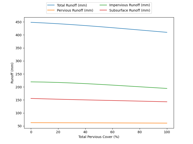
Figure 2.4 % change in surface runoff plotted with tree cover %
Impervious Cover Effects
Impervious cover has a significant impact in the mitigation of runoff - approximately a 20 times increase in runoff compared to the same changes in tree cover. Impervious surfaces affect both the velocity and volume of water, with the base flow, and thereby infiltration, decreasing to 0 at 100% impervious cover.
Removal of all impervious cover at the shoreline of the Black subbasin would decrease runoff during the simulation period by an average of -69.77% (-0.16 million m3). An increase in impervious cover from 36.0 to 100% would increase runoff by 412.62% (0.97 million m3) during the 12-month simulation period.
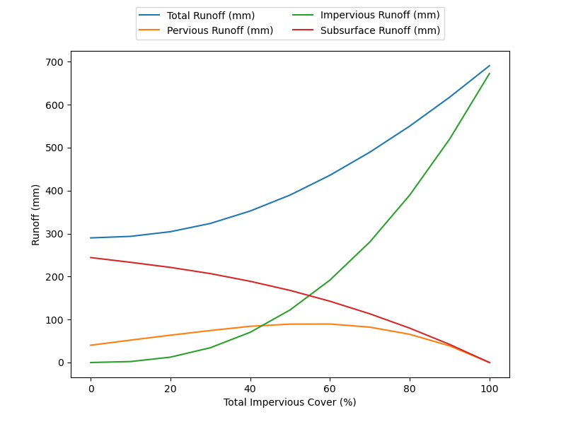
Figure 2.5 % change in surface runoff plotted with impervious cover %
Cumulative Effects

Figure 2.6 Changes in runoff during simulation period based on changes in percent impervious and percent tree cover. Black ‘+’ represents current conditions.
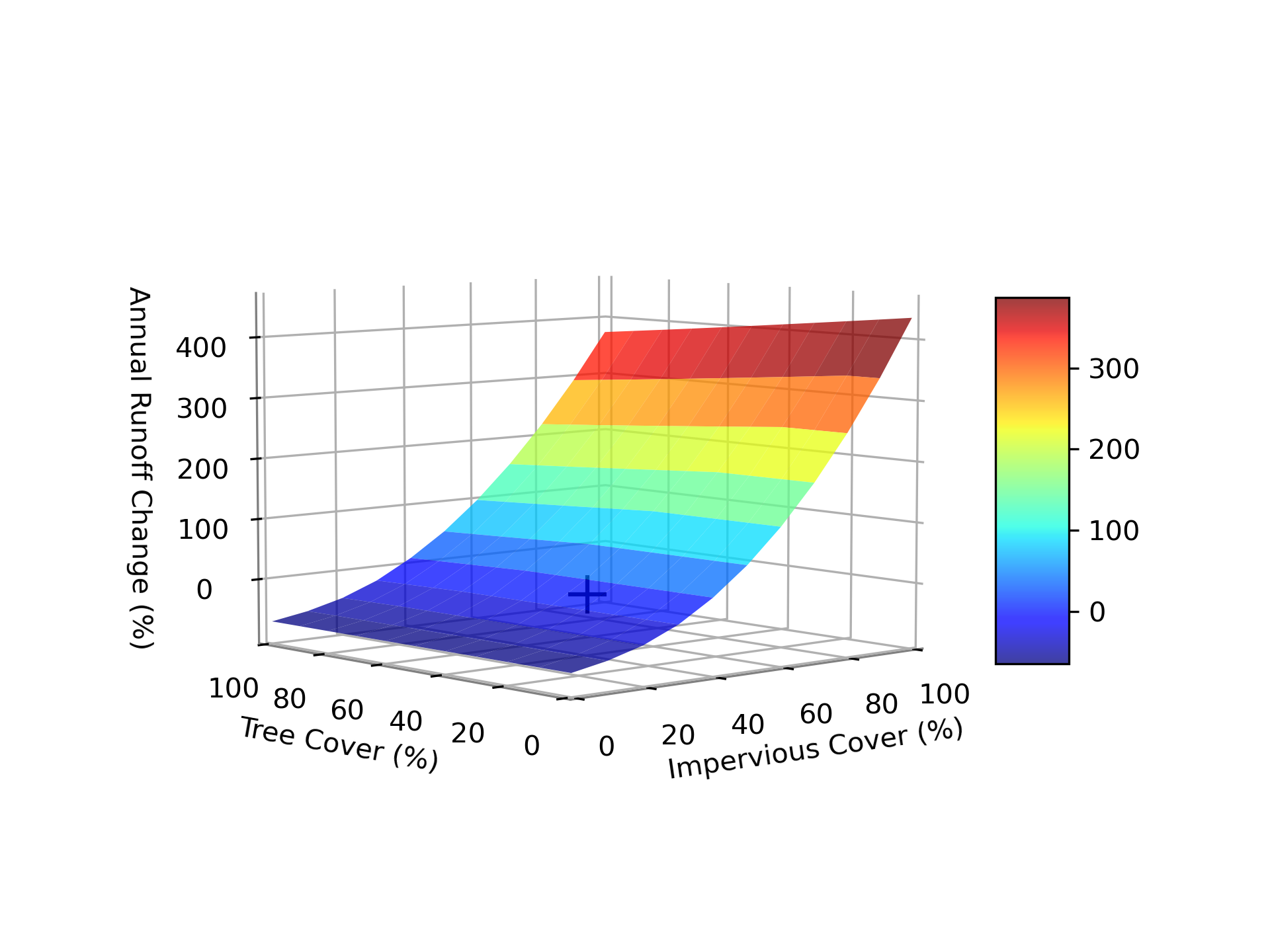
Figure 2.7 Percent change in annual runoff during simulation period based on changes in percent impervious and percent tree cover. Black ‘+’ represents current conditions.
During the simulation period the total rainfall recorded was 805.18. Since that amount is assumed to have fallen over the entire 1.76 watershed, a total of 1415989.5479999995 m3 of rain fell on the watershed during the simulation period. The total stream flow modeled for the simulation period in the base case scenario (no land cover change) was 0.23 million m3. The stream flow is made up of runoff and baseflow. The greatest contribution to stream flow was runoff from pervious areas, which was estimated to generate 2.47% of stream flow. Baseflow and runoff from impervious areas generated 59.12% and 21.22% of stream flow respectively (Figure 2.8).
Watershed areas with tree canopy intercepted about 21.67% of the rainfall that fell in those areas; but as only 35.0% of the watershed is under tree canopy, interception of total precipitation by trees was only 7.59% (107404.07 m3). Watershed areas with short vegetation cover (grasses and herbaceous vegetation) intercepted about 9.95% of the rainfall that fell in those areas; but as only 29.0% of the watershed has short vegetation cover, interception of total precipitation by short vegetation was only 2.88% (40846.85 m3).
Effects on Water Quality
Based on the changes in runoff rates and the EMC values used (Table 2.3), the current tree cover is estimated to reduce total suspended solids during the simulation period by about 137.98 kilograms.
| Total Suspended Solids | Total Phosphorus | Total Nitrogen | |
| Median | 130.86 | 0.1878 | 2.32 |
Table 2.8 Localized pollutant coefficients (mg/L) based on White et al. (2015) and Stephan et al. (2017).
Discussion
The health of shorelines is critically important for providing a buffer from phosphorus, nitrogen, and sediment-rich runoff to the Great Lakes, as well as preventing erosion and shoreline degradation from the lakes. The shorelines of the Great Lakes are mostly undeveloped, playing a key role in nutrient cycling, sediment transport, and wildlife habitat. In developing best management practices (BMPs), maintaining the natural environment while stabilizing shorelines and private properties must all be considered.
Considering the low development of the Great Lakes shoreline, emphasis should be placed on adding tree cover to impervious land as opposed to removing impervious cover or adding impervious cover to pervious land. Tree canopy intercepts about 2.5 times more rainfall than short vegetation – maximizing the leaf area over impervious surfaces or areas with high pollutant loading would maximize the reduction in stormwater runoff quality and quantity.
This report is meant to provide a broad overview of the shoreline area of the Black subbasin, and understand the impacts of tree and impervious cover on runoff, stream flow, and water quality. Through informed landscape designs focused on land use and tree cover, runoff can be reduced, and water quality improved over surfaces and in waterways that drain directly into the Great Lakes.
Nutrient Loading
Data and Methods
The i-Tree Buffer model is built upon the framework of Endreny and Wood (2003) and creates maps of watershed runoff likelihood and buffering likelihood values. This analysis used publicly available GIS inputs, annual rainfall data, and local (White et al., 2015) values for nonpoint source (NPS) loading of nutrients. The GIS inputs include digital elevation model (DEM) data and land use data, retrieved from NHDPlusV2 and National Land Cover Database (NLCD), respectively.
Values for NPS loading were taken from compiled look-up tables of local export coefficient (EC, kg/ha/yr) values (Table 3.1) developed by White et al. (2015), which estimated water quality data at the HUC-8 basin scale nationwide based on 45 million stochastic Soil and Water Assessment Tool (SWAT) simulations. ECs represent the annual loads of a pollutant for a given land cover type, and are empirically derived from observed water quality data from catchments with varying land uses. Land cover types representing permanent water or ice (NLCD classes 11, 12, 90, and 95) were assumed to have ECs of zero.
| Pollutant | NLCDa | 5th percentile | 10th percentile | 25th percentile | 50th percentile | 75th percentile | 90th percentile |
|---|---|---|---|---|---|---|---|
| TP | 21 | 2.354 | 2.79 | 3.709 | 4.888 | 5.696 | 6.264 |
| 22 | 2.354 | 2.79 | 3.709 | 4.888 | 5.696 | 6.264 | |
| 23 | 2.354 | 2.79 | 3.709 | 4.888 | 5.696 | 6.264 | |
| 24 | 2.354 | 2.79 | 3.709 | 4.888 | 5.696 | 6.264 | |
| 41 | 0.0 | 0.0 | 0.098 | 0.136 | 0.165 | 0.201 | |
| 42 | 0.0 | 0.0 | 0.098 | 0.136 | 0.165 | 0.201 | |
| 43 | 0.0 | 0.0 | 0.098 | 0.136 | 0.165 | 0.201 | |
| 71 | 0.007 | 0.019 | 0.045 | 0.09 | 0.162 | 0.37 | |
| 81 | 1.027 | 1.327 | 1.993 | 3.131 | 4.59 | 5.922 | |
| 82 | 5.489 | 6.752 | 8.939 | 11.561 | 14.43 | 17.119 | |
| TN | 21 | 32.775 | 36.86 | 44.953 | 54.503 | 60.705 | 65.245 |
| 22 | 32.775 | 36.86 | 44.953 | 54.503 | 60.705 | 65.245 | |
| 23 | 32.775 | 36.86 | 44.953 | 54.503 | 60.705 | 65.245 | |
| 24 | 32.775 | 36.86 | 44.953 | 54.503 | 60.705 | 65.245 | |
| 41 | 2.062 | 2.3 | 2.763 | 3.489 | 4.44 | 5.457 | |
| 42 | 2.062 | 2.3 | 2.763 | 3.489 | 4.44 | 5.457 | |
| 43 | 2.062 | 2.3 | 2.763 | 3.489 | 4.44 | 5.457 | |
| 71 | 0.846 | 1.09 | 1.59 | 2.311 | 3.727 | 6.88 | |
| 81 | 17.036 | 20.864 | 28.178 | 38.973 | 53.189 | 66.427 | |
| 82 | 50.9 | 63.304 | 80.454 | 100.801 | 122.624 | 145.661 |
Table 3.1 Export coefficients based on percentile and pollutant type (White et al. 2015)
a NLCD land cover classes: 21 - Developed, open space; 22 - Developed, low intensity; 23 - Developed, medium intensity;
24 - Developed, high intensity; 41 - Deciduous forest; 42 - Evergreen forest; 43 - Mixed forest; 71 - Grassland or herbaceous; 81 - Pasture or hay; 82 - Cultivated crops
With these input data, the model calculated:
separate ECs for each pixel;
a separate surface and subsurface runoff index (RI) for each pixel based on the fractions of impervious and pervious area in each upslope contributing area pixel, which is related to an estimate of surface and subsurface wetness; and
a separate surface and subsurface buffer index (BI) for each pixel based on flow resistance and potential energy, which is related to runoff velocity and an estimate of NPS buffering in downslope dispersal area pixels.
The entire set of pixel specific RI and BI values are normalized to the watershed mean RI and BI values (or median values, depending on user preference), and multiplied by the land cover EC to quantify pollutant loading likelihood. In this way i-Tree Buffer treats pollutant loading as spatially variant, depending on both RI from upslope pixels and BI from downslope pixels. As demonstrated in Figure 2.1, changes in RI and BI control pollutant loading through changes in runoff magnitude (i.e., size of arrows under each scenario) and/or pollutant concentration (i.e., the color of arrows under each scenario).

Figure 3.2 Conceptual model of the effects of contributing area RI (a & b) and dispersal area BI (c & d) on NPS loading from a pixel of interest.
Weighted surface and subsurface EC values for each pixel i, or dynamic export coefficients (ECd), are calculated as:
$$EC_{d,surf,i} = EC_{surf,i}*\frac{RI_{surf,i}}{RI_{surf,avg}}*\frac{BI_{surf,avg}}{BI_{surf,i}}$$
(Eq. 1)
$$EC_{d,sub,i} = EC_{sub,i}*\frac{RI_{sub,i}}{RI_{sub,avg}}*\frac{BI_{sub,avg}}{BI_{sub,i}}$$
(Eq. 2)
where ECi represents the unweighted EC (kg/ha/yr) for land cover type i, RIi is the pixel’s surface or subsurface runoff index value, the RIavg is the corresponding average surface or subsurface runoff index in the watershed, the BIi is the pixel’s surface or subsurface buffer index value, and BIavg is the corresponding average surface or subsurface buffer index in the watershed. The NPS pollutant of phosphorus was simulated as total phosphorus entrained in surface runoff processes, denoted as ECsurf,i in Equation 1. The NPS pollutant of nitrogen was simulated as dissolved total nitrogen in subsurface runoff processes, denoted as ECsub,i in Equation 2 (Stephan and Endreny 2016).
Values of ECd for P and N were calculated for the entire watershed and mapped in 30m square pixels. To focus on the most critical watershed areas for possible management and remediation, three hotspots were identified in the watershed for TN, TP, and TSS. Hotspots were calculated by a moving 3x3 window of 30m cells, with a 0.5 km buffer in each direction. In other words, hotspots were gathered by the 3x3 cell average, with no hotspot less than 0.5km away from each other.
Results
Effects of Land Use on Water Quality
Based on the current and potential land use, event mean concentrations (EMCs) were calculated based on White et al. (2015) and plotted into ternary heat maps.
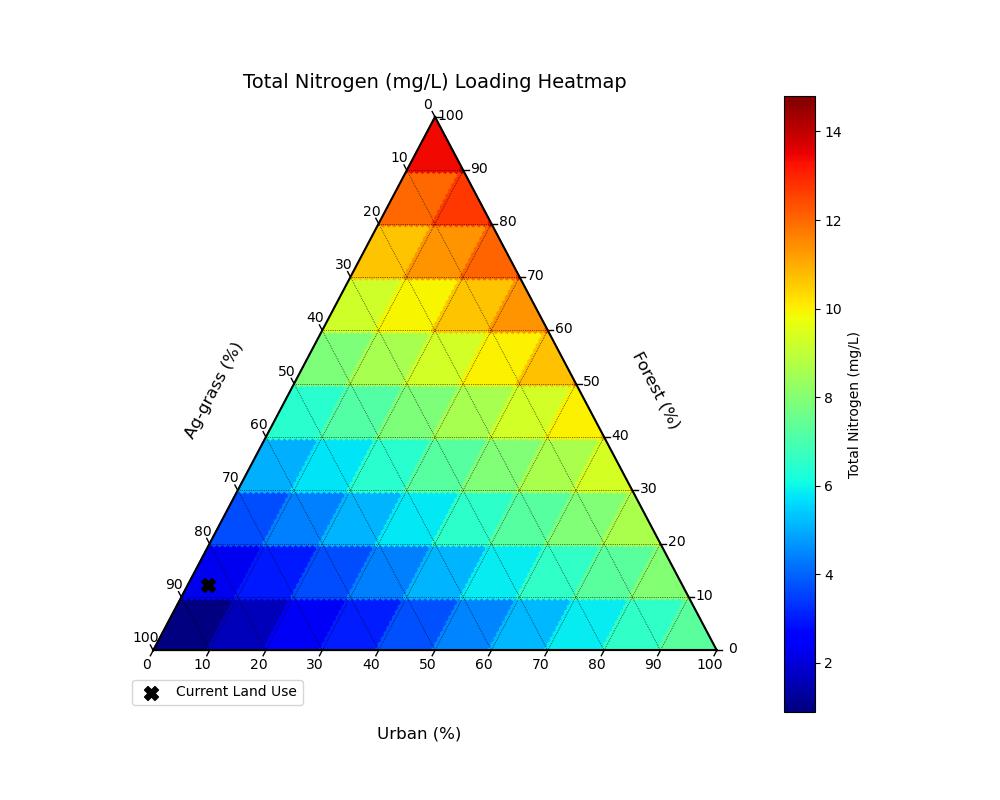
Figure 3.3: Localized pollutant coefficients (mg/L) for Total Nitrogen based on White et al. (2015). Black 'X' represents current conditions.
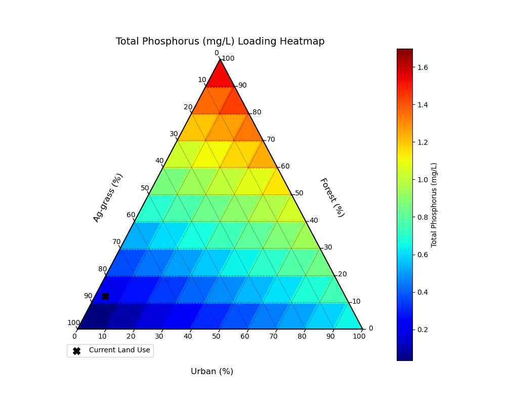
Figure 3.4: Localized pollutant coefficients (mg/L) for Total Phosphorus based on White et al. (2015). Black 'X' represents current conditions.
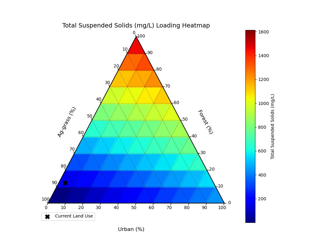
Figure 3.5 Localized pollutant coefficients (mg/L) for Total Suspended Solids based on White et al. (2015). Black 'X' represents current conditions.
Hotspots
The watershed mean loading value was 41.28 kg/ha/yr of total nitrogen (TN) and the standard deviation was 117.87 kg/ha/yr.
Explore the top hotspots for total nitrogen (TN) below:
Or view the images and coordinates for the top 3 hotspots:
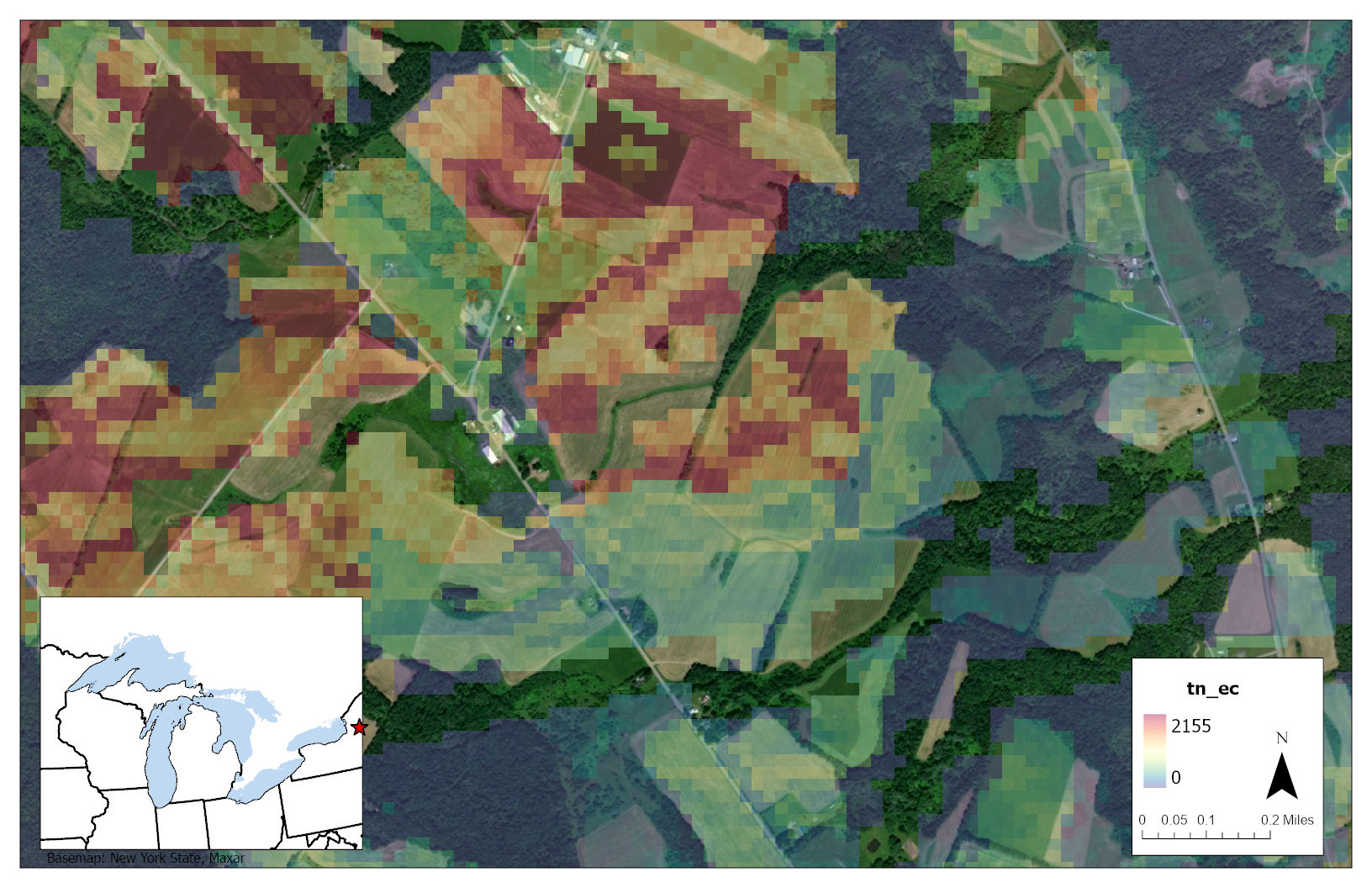
Figure 3.6 Hotspot 1: Latitude:43.66197 Longitude:-75.40512
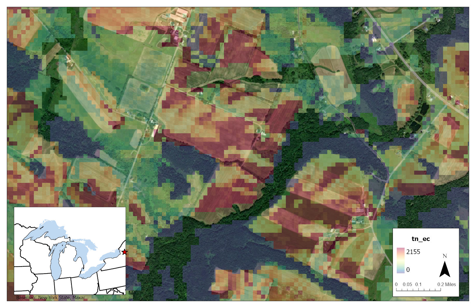
Figure 3.7 Hotspot 2: Latitude:43.69695 Longitude:-75.41737
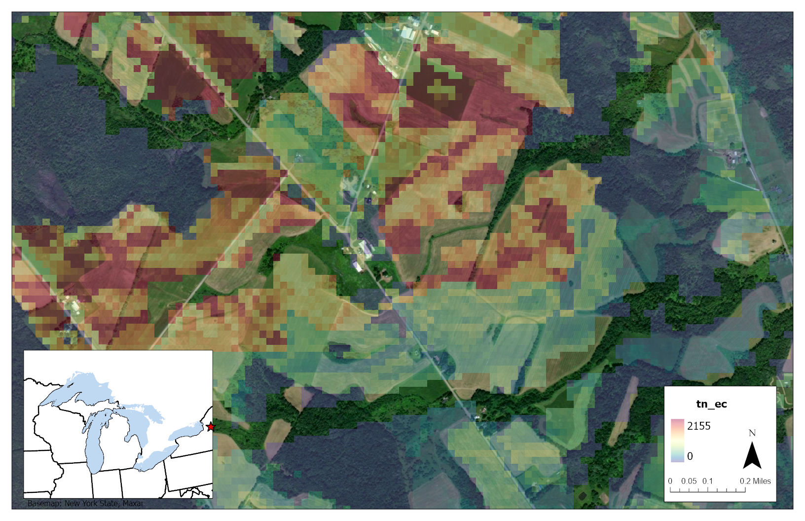
Figure 3.8 Hotspot 3: Latitude:43.66255 Longitude:-75.40877
The watershed mean loading value was 3.83 kg/ha/yr of total phosphorus (TP) and the standard deviation was 12.6 kg/ha/yr.
Explore the top hotspots for total phosphorus (TP) below:
Or view the images and coordinates for the top 3 hotspots:
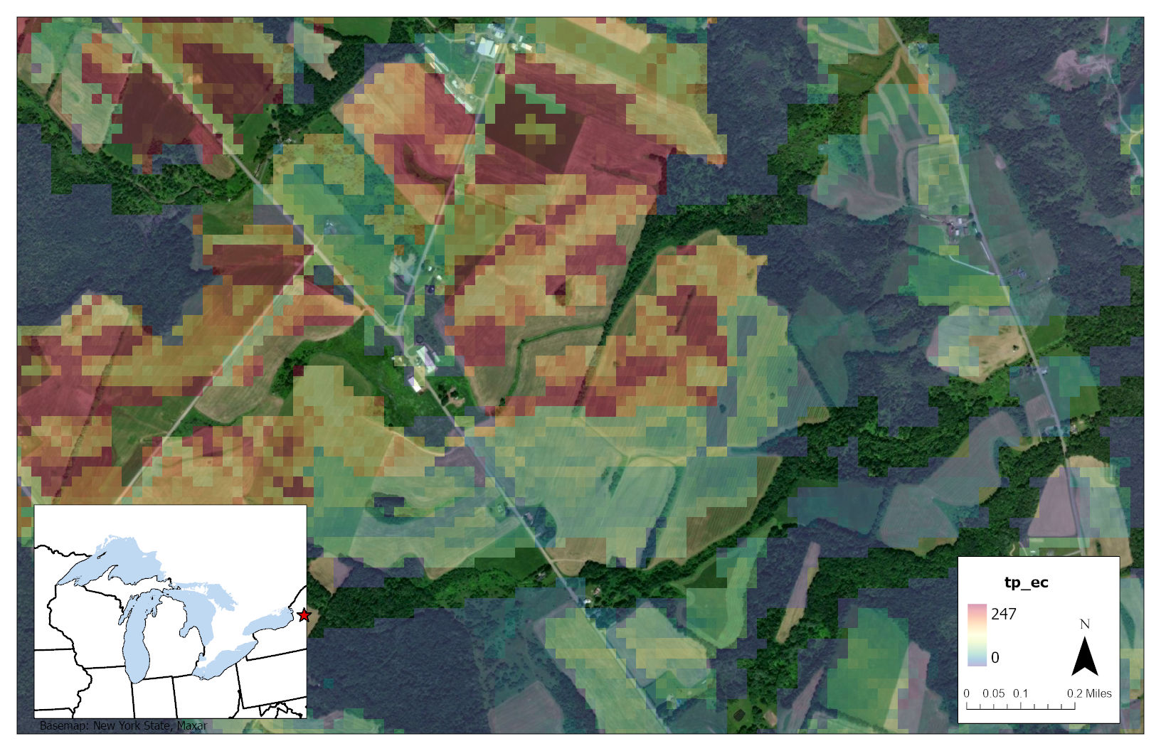
Figure 3.9 Hotspot 1: Latitude:43.66197 Longitude:-75.40512
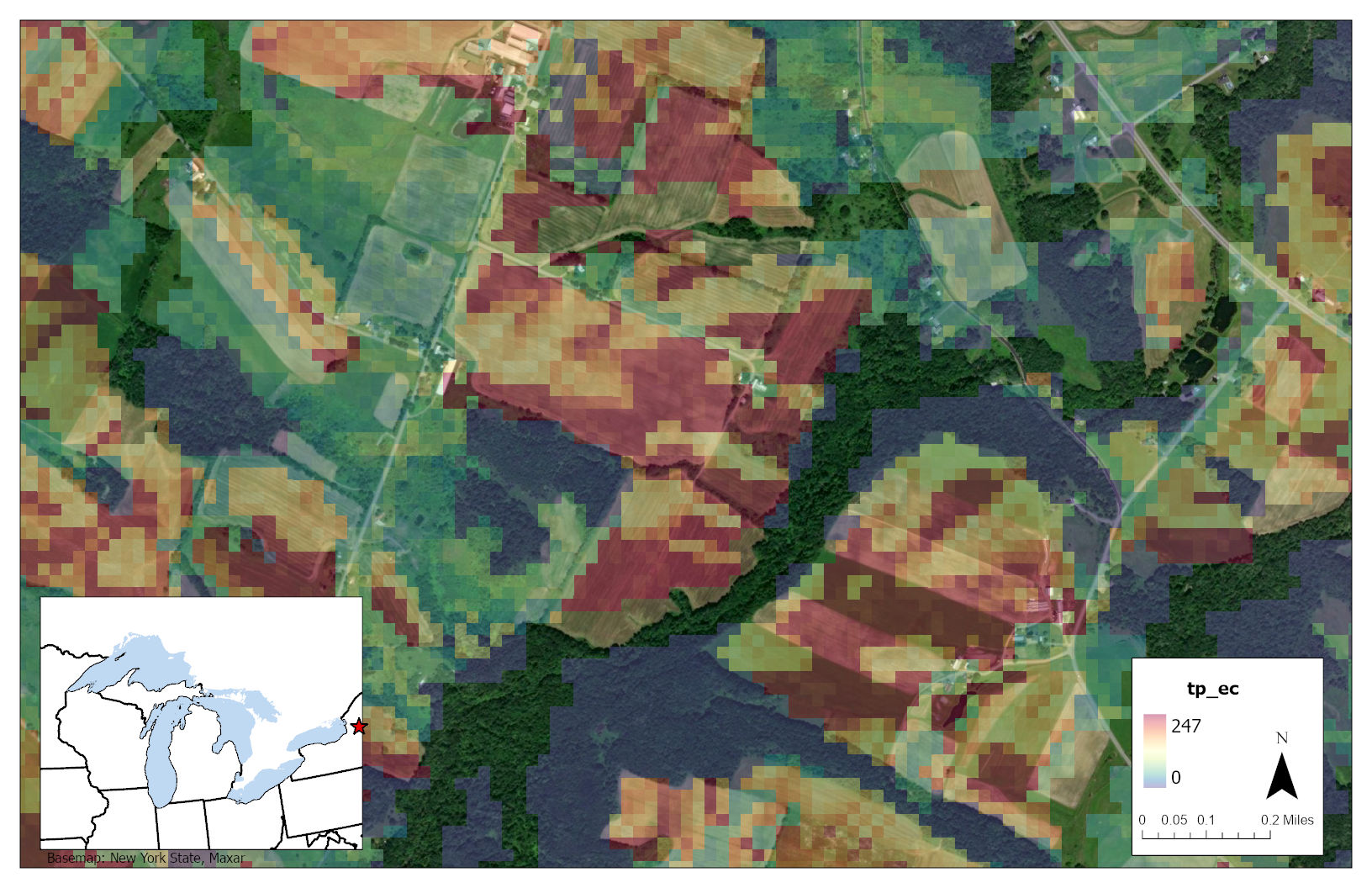
Figure 3.10 Hotspot 2: Latitude:43.69695 Longitude:-75.41737
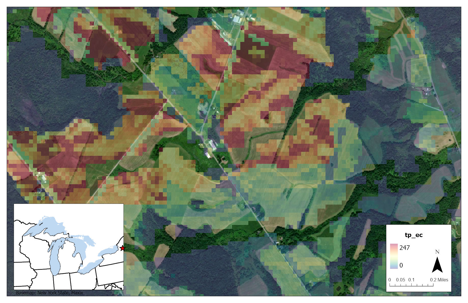
Figure 3.11 Hotspot 3: Latitude:43.66255 Longitude:-75.40877
Discussion
The resolution of the ECd result rasters is constrained by the coarse resolution of the input data, but Buffer can run with 30m pixels and produce maps with useful insight into trends of RI, BI, and ECd. The 30m input data captures flow path tendency toward perennial stream networks while maintaining this study’s first-order modeling approach and providing results closer to the scales at which remediation designs are implemented. For urban basins in particular, the model accuracy can be improved if used with higher resolution elevation and land cover data, since coarser data can miss sub-pixel details of land use and flow paths imposed by features such as road crowns and curbs. However, although Stephan and Endreny (2016) ultimately used <1m input data they saw <1% difference in total nutrient load values between 0.3m and 10m grid sizes.
For each of the critical hotspots, management efforts to reduce NPS nutrient loading could take one of several approaches. General approaches can be divided into three categories:
- Reducing pollutant export at the hotspot. This reduction could involve altering land cover at the hotspot to land cover with a lower NPS loading value or incorporating best management practices into the current land use (e.g., contour farming and covered fertilizer storage in an agricultural hotspot).
- Increasing buffering capacity in the downslope flow path of the hotspot (i.e. raising BI). BI values increase with increasing water travel times in the downslope dispersal area. Travel times could be increased by increasing the percentages of herbaceous and woody vegetation in dispersal area land cover, or by decreasing local terrain slopes.
- Reducing runoff generation upslope of the hotspot (i.e. lowering RI). This reduction could be accomplished by removing impervious cover or decreasing local terrain slopes in the upslope contributing area.
A management plan for a given hotspot could involve any combination of the above approaches. Ultimately, management needs to be tailored to each hotspot’s unique conditions for land cover and land use, topographic index, social conditions, and plantable space. Trees and forests help reduce NPS nutrients through any of the three approaches listed above when planted in the right place for the right reason. These trees would also provide many co-benefits and contribute to sustainable forestry, agroforestry, and ecosystem restoration in these hotspot areas.
All of these management approaches could be further directed by taking plantable space into account. Nutrient hotspot locations can be compared with local plantable space data to strategically target tree plantings that will minimize NPS pollution as well as expand tree canopy in low-canopy areas. Strategic planting of trees has been identified as a crucial component of reducing NPS pollution in both urban and rural watersheds (Sharpley et al., 2006; Hynicka and Caraco, 2017).